Quant II Recitation

Drew Dimmery

January 30, 2015

What is this?

This presentation created using knitr + pandoc + reveal.js
I have created a recitation repository on github: https://github.com/ddimmery/Quant-II-Recitation
The recitation website will also be on github, at http://ddimmery.github.io/Quant-II-Recitation
This presentation is available on the course website, as is a handout version in pdf.
The raw .Rmd file is available in the repository. You can create a handout version of it with the following commands (assuming knitr and pandoc are installed), first in R:
```
require(knitr)
knit(presentation.Rmd)
```
And then on the command line:
```
pandoc presentation.md -o handout.pdf
```

Today’s Topic

Sharing is caring.
- If you don’t share your research (+ code and data) then what’s the point of doing it?
Today we will be discussing some necessary mechanics.
- R and how to bend it to your will
- Producing high quality tables / plots
- If there’s any time left, we can talk a little more about identification

Workflow

Find an editor and learn everything about it:
- vim (+ Vim-R-plugin)
- emacs (+ ESS [Emacs Speaks Statistics])
- Notepad++, Kate, Sublime, etc
- Rstudio
- Eclipse (+ StatET)
Familiarize yourself with version control software
- git (github or TortoiseGit)
- or just Dropbox

When things break

Documentation - Ex: ?lm
Google
CRAN (Reference manuals, vignettes, etc) - Ex: http://cran.r-project.org/web/packages/AER/index.html
JSS - Ex: http://www.jstatsoft.org/v27/i02
Stack Overflow - http://stackoverflow.com/questions/tagged/r
Listservs - http://www.r-project.org/mail.html

Resources

The Art of R Programming - N. Matloff
Modern Applied Statistics with S - W. Venables and B. Ripley
Advanced R Programming - forthcoming, H. Wickham
The R Inferno - P. Burns
Rdataviz - a talk by P. Barberá on ggplot2
Basic Intro to R - also by P. Barberá

Reading R Documentation

?lm

CRAN documentation

JSS

plm

Confusing Things

At the prompt, > means you’re good to go, + means a parenthesis or bracket is open.
Case sensitive
Use / in path names. Not \.
R uses variables – there is no “sheet” here, like in Stata
R is a programming language
More on errors later!

Using Third-party Code

Relevant commands are: install.packages and library

Find the appropriate packages and commands with Google and via searching in R:

?covariance
??covariance
install.packages("sandwich")
library("sandwich")
?vcovHC

Data types

Character - strings
Double / Numeric - numbers
Logical - true/false
Factor - unordered categorical variables
Objects - its complicated

Character

str <- "This is a string"

paste("This", "is", "a", "string", sep = " ")

## [1] "This is a string"

as.character(99)

## [1] "99"

class(str)

## [1] "character"

Numeric

num <- 99.867
class(num)

## [1] "numeric"

round(num, digits = 2)

## [1] 99.87

round(str, digits = 2)

## Error: non-numeric argument to mathematical function

pi

## [1] 3.142

exp(1)

## [1] 2.718

sin, exp, log, factorial, choose, BesselJ, etc

Logical

The logical type allows us to make statements about truth

2 == 4

## [1] FALSE

class(2 == 4)

## [1] "logical"

str != num

## [1] TRUE

"34" == 34

## [1] TRUE

==, !=, >, <, >=, <=, !, &, |, any, all, etc

Objects

Many functions will return objects rather than a single datatype.

X <- 1:100
Y <- rnorm(100, X)
out.lm <- lm(Y ~ X)
class(out.lm)

## [1] "lm"

Objects can have other data embedded inside them

out.lm$rank

## [1] 2

class(out.lm$rank)

## [1] "integer"

Data Structures

There are other ways to hold data, though:
- Vectors
- Lists
- Matrices
- Dataframes

Vectors

Almost everything in R is a vector.

as.vector(4)

## [1] 4

## [1] 4

We can combine vectors with c:

vec <- c("a", "b", "c")
vec

## [1] "a" "b" "c"

c(2, 3, vec)

## [1] "2" "3" "a" "b" "c"

Vectors (cont.)

Sometimes R does some weird stuff:

c(1, 2, 3, 4) + c(1, 2)

## [1] 2 4 4 6

It “recycles” the shorter vector:

c(1, 2, 3, 4) + c(1, 2, 1, 2)

## [1] 2 4 4 6

c(1, 2, 3, 4) + c(1, 2, 3)

## Warning: longer object length is not a multiple of shorter object length

## [1] 2 4 6 5

More Vectors

We can index vectors in several ways

vec[1]

## [1] "a"

names(vec) <- c("first", "second", "third")
vec

##  first second  third 
##    "a"    "b"    "c"

vec["first"]

## first 
##   "a"

Missingness

vec[1] <- NA
vec

##  first second  third 
##     NA    "b"    "c"

is.na(vec)

##  first second  third 
##   TRUE  FALSE  FALSE

vec[!is.na(vec)]  # vec[complete.cases(vec)]

## second  third 
##    "b"    "c"

Lists

Lists are similar to vectors, but they allow for arbitrary mixing of types and lengths.

listie <- list(first = vec, second = num)
listie

## $first
##  first second  third 
##     NA    "b"    "c" 
## 
## $second
## [1] 99.87

listie[[1]]

##  first second  third 
##     NA    "b"    "c"

listie$first

##  first second  third 
##     NA    "b"    "c"

Matrices

\[A = \begin{pmatrix}1 & 3\\ 2 & 4\end{pmatrix}\]
\(A_{ij}\)
\(A_{1,2} = 3\)
\(A_{1,\cdot} = (1,3)\)

A <- matrix(c(1, 2, 3, 4), nrow = 2, ncol = 2)
A

##      [,1] [,2]
## [1,]    1    3
## [2,]    2    4

A[1, 2]

## [1] 3

A[1, ]

## [1] 1 3

Matrix Operations

Its very easy to manipulate matrices:

solve(A)  #A^{-1}

##      [,1] [,2]
## [1,]   -2  1.5
## [2,]    1 -0.5

10 * A

##      [,1] [,2]
## [1,]   10   30
## [2,]   20   40

B <- diag(c(1, 2))
B

##      [,1] [,2]
## [1,]    1    0
## [2,]    0    2

A %*% B

##      [,1] [,2]
## [1,]    1    6
## [2,]    2    8

More Matrix Ops.

A %*% diag(3)

## Error: non-conformable arguments

t(A)  # A'

##      [,1] [,2]
## [1,]    1    2
## [2,]    3    4

rbind(A, B)

##      [,1] [,2]
## [1,]    1    3
## [2,]    2    4
## [3,]    1    0
## [4,]    0    2

cbind(A, B)

##      [,1] [,2] [,3] [,4]
## [1,]    1    3    1    0
## [2,]    2    4    0    2

c(1, 2, 3) %x% c(1, 1)  # Kronecker Product

## [1] 1 1 2 2 3 3

Naming Things

rownames(A)

## NULL

rownames(A) <- c("a", "b")
colnames(A) <- c("c", "d")
A

##   c d
## a 1 3
## b 2 4

A[, "d"]

## a b 
## 3 4

Matrices are vectors:

A[3]

## [1] 3

Dataframes

The workhorse
Basically just a matrix that allows mixing of types.

data(iris)
head(iris)

##   Sepal.Length Sepal.Width Petal.Length Petal.Width Species
## 1          5.1         3.5          1.4         0.2  setosa
## 2          4.9         3.0          1.4         0.2  setosa
## 3          4.7         3.2          1.3         0.2  setosa
## 4          4.6         3.1          1.5         0.2  setosa
## 5          5.0         3.6          1.4         0.2  setosa
## 6          5.4         3.9          1.7         0.4  setosa

Control Flow

loops
if/else
functions
useful stock functions to know

Loops

for loops - just a way to say “do this for each element of the index”
“this” is defined in what follows the “for” expression

for (i in 1:5) {
    cat(i * 10, " ")
}

## 10  20  30  40  50

for (i in 1:length(vec)) {
    cat(vec[i], " ")
}

## NA  b  c

for (i in vec) {
    cat(i, " ")
}

## NA  b  c

If/Else

if (vec[2] == "b") print("Hello World!")

## [1] "Hello World!"

if (vec[3] == "a") {
    print("Hello World!")
} else {
    print("!dlroW olleH")
}

## [1] "!dlroW olleH"

Vectorized If/Else

Conditional execution on each element of a vector

vec <- letters[1:3]
new <- vector(length = length(vec))
for (i in 1:length(vec)) {
    if (vec[i] == "b") {
        new[i] <- 13
    } else {
        new[i] <- 0
    }
}
new

## [1]  0 13  0

new <- ifelse(vec == "b", 13, 0)
new

## [1]  0 13  0

Functions

\(f : X \to Y\)
Functions in R are largely the same. (“Pure functions”)

add3 <- function(X) {
    return(X + 3)
}
add3(2)

## [1] 5

makeGroups <- function(groups, members = 1) {
    return((1:groups) %x% rep(1, members))
}
makeGroups(5)

## [1] 1 2 3 4 5

makeGroups(5, 2)

##  [1] 1 1 2 2 3 3 4 4 5 5

Useful Functions

Note: Most functions don’t do complete case analysis by default (usually option na.rm=TRUE)
print, cat, paste, with, length, sort, order, unique, rep, nrow, ncol, complete.cases, subset, merge, mean, sum, sd, var, lag,lm, model.matrix,coef, vcov, residuals, vcovHC (from sandwich), ivreg (from AER), countrycode (fromcountrycode),summary, pdf, plot, Tools from plm, and many more.

Distributional Functions

?Distributions
They have a consistent naming scheme.
rnorm, dnorm, qnorm, pnorm
rdist - generate random variable from dist
ddist - density function of dist
qdist - quantile function of dist
pdist - distribution function of dist
look at documentation for parameterization

rnorm(16)

##  [1]  0.03219 -0.89729 -0.28782  0.86993 -1.21937  1.47985  0.38488
##  [8]  0.28917 -1.66721  0.23155  1.63280  0.84529 -0.87946 -0.22374
## [15]  1.35861 -0.61532

Robust SEs

robust.se <- function(model,cluster=1:length(model$residuals)) {
  require(sandwich)
  require(lmtest)
  M <- length(unique(cluster))
  N <- length(cluster)
  K <- model$rank
  dfc <- (M/(M - 1)) * ((N - 1)/(N - K))
  uj  <- apply(
               estfun(model),
               2,
               function(x) tapply(x, cluster, sum)
              )
  rcse.cov <- dfc * sandwich(model,meat = crossprod(uj)/N)
  rcse.se <- coeftest(model, rcse.cov)
  return(list(rcse.cov, rcse.se))
}

Multiple Dispactch

Sometimes functions will behave differently based on context:

summary(vec)

##    Length     Class      Mode 
##         3 character character

summary(c(1, 2, 3, 4))

##    Min. 1st Qu.  Median    Mean 3rd Qu.    Max. 
##    1.00    1.75    2.50    2.50    3.25    4.00

summary(iris[, 1:4])

##   Sepal.Length   Sepal.Width    Petal.Length   Petal.Width 
##  Min.   :4.30   Min.   :2.00   Min.   :1.00   Min.   :0.1  
##  1st Qu.:5.10   1st Qu.:2.80   1st Qu.:1.60   1st Qu.:0.3  
##  Median :5.80   Median :3.00   Median :4.35   Median :1.3  
##  Mean   :5.84   Mean   :3.06   Mean   :3.76   Mean   :1.2  
##  3rd Qu.:6.40   3rd Qu.:3.30   3rd Qu.:5.10   3rd Qu.:1.8  
##  Max.   :7.90   Max.   :4.40   Max.   :6.90   Max.   :2.5

Why? ?summary ?summary.lm

The *apply family

These functions allow one to efficiently perform a large number of actions on data.
apply - performs actions on the rows or columns of a matrix/array (1 for rows, 2 for columns, 3 for ??)
sapply - performs actions on every element of a vector
tapply - performs actions on a vector by group
replicate - performs the same action a given number of times

apply

##   c d
## a 1 3
## b 2 4

apply(A, 1, sum)

## a b 
## 4 6

apply(A, 2, mean)

##   c   d 
## 1.5 3.5

sapply

vec

## [1] "a" "b" "c"

sapply(vec, function(x) paste0(x, ".vec"))

##       a       b       c 
## "a.vec" "b.vec" "c.vec"

Can be accomplished more simply with:

paste0(vec, ".vec")

## [1] "a.vec" "b.vec" "c.vec"

Why?
replicate is basically just sapply(1:N,funct) where funct never uses the index.

tapply

tapply(1:10, makeGroups(5, 2), mean)

##   1   2   3   4   5 
## 1.5 3.5 5.5 7.5 9.5

Working With Data

Input
Output

Input

setwd("~/github/Quant II Recitation/2014-01-31/")
dir()

## [1] "apsrtable.png"     "figure"            "handout.pdf"      
## [4] "iris.csv"          "presentation.html" "presentation.md"  
## [7] "presentation.Rmd"  "stargazer.png"

iris <- read.csv("iris.csv")

If data is, for instance, a Stata .dta file, use read.dta from the foreign package.
Useful options for reading data: sep, na.strings, stringsAsFactors
For different formats, Google it.

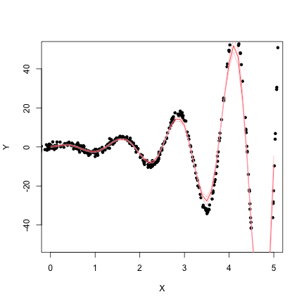
Simulate some Data

set.seed(1023)  # Important for replication
X <- rnorm(1000, 0, 5)
Y <- sin(5 * X) * exp(abs(X)) + rnorm(1000)
dat <- data.frame(X, Y)
plot(X, Y, xlim = c(0, 5), ylim = c(-50, 50))

Regression Output

dat.lm <- lm(Y ~ X, data = dat)
dat.lm

## 
## Call:
## lm(formula = Y ~ X, data = dat)
## 
## Coefficients:
## (Intercept)            X  
##     -216634       183687

Regression Output

summary(dat.lm)

## 
## Call:
## lm(formula = Y ~ X, data = dat)
## 
## Residuals:
##       Min        1Q    Median        3Q       Max 
## -2.10e+08 -4.19e+05  2.01e+05  8.17e+05  9.08e+06 
## 
## Coefficients:
##             Estimate Std. Error t value Pr(>|t|)    
## (Intercept)  -216634     212126   -1.02     0.31    
## X             183687      43470    4.23  2.6e-05 ***
## ---
## Signif. codes:  0 '***' 0.001 '**' 0.01 '*' 0.05 '.' 0.1 ' ' 1
## 
## Residual standard error: 6710000 on 998 degrees of freedom
## Multiple R-squared:  0.0176, Adjusted R-squared:  0.0166 
## F-statistic: 17.9 on 1 and 998 DF,  p-value: 2.6e-05

Pretty Output

How do we get LaTeX output?
The xtable package:

require(xtable)

## Loading required package: xtable

xtable(dat.lm)

## % latex table generated in R 3.0.2 by xtable 1.7-1 package
## % Tue Jan 28 23:38:40 2014
## \begin{table}[ht]
## \centering
## \begin{tabular}{rrrrr}
##   \hline
##  & Estimate & Std. Error & t value & Pr($>$$|$t$|$) \\ 
##   \hline
## (Intercept) & -216633.6722 & 212125.4622 & -1.02 & 0.3074 \\ 
##   X & 183687.1735 & 43469.5839 & 4.23 & 0.0000 \\ 
##    \hline
## \end{tabular}
## \end{table}

xtable

xtable works on any sort of matrix

xtable(A)

## % latex table generated in R 3.0.2 by xtable 1.7-1 package
## % Tue Jan 28 23:38:40 2014
## \begin{table}[ht]
## \centering
## \begin{tabular}{rrr}
##   \hline
##  & c & d \\ 
##   \hline
## a & 1.00 & 3.00 \\ 
##   b & 2.00 & 4.00 \\ 
##    \hline
## \end{tabular}
## \end{table}

xtable

This is what xtable does with the lm object:

class(summary(dat.lm)$coefficients)

## [1] "matrix"

xtable(summary(dat.lm)$coefficients)

## % latex table generated in R 3.0.2 by xtable 1.7-1 package
## % Tue Jan 28 23:38:40 2014
## \begin{table}[ht]
## \centering
## \begin{tabular}{rrrrr}
##   \hline
##  & Estimate & Std. Error & t value & Pr($>$$|$t$|$) \\ 
##   \hline
## (Intercept) & -216633.67 & 212125.46 & -1.02 & 0.31 \\ 
##   X & 183687.17 & 43469.58 & 4.23 & 0.00 \\ 
##    \hline
## \end{tabular}
## \end{table}

Note that this is the same as the output from xtable(dat.lm)

Pretty it up

Now let’s make some changes to what xtable spits out:

print(xtable(dat.lm, digits = 1), booktabs = TRUE)

## % latex table generated in R 3.0.2 by xtable 1.7-1 package
## % Tue Jan 28 23:38:40 2014
## \begin{table}[ht]
## \centering
## \begin{tabular}{rrrrr}
##   \toprule
##  & Estimate & Std. Error & t value & Pr($>$$|$t$|$) \\ 
##   \midrule
## (Intercept) & -216633.7 & 212125.5 & -1.0 & 0.3 \\ 
##   X & 183687.2 & 43469.6 & 4.2 & 0.0 \\ 
##    \bottomrule
## \end{tabular}
## \end{table}

Many more options, see ?xtable and ?print.xtable

apsrtable

Read the documentation - there are many options.

require(apsrtable)

## Loading required package: apsrtable

dat.lm2 <- lm(Y ~ X + 0, data = dat)
apsrtable(dat.lm, dat.lm2)

## Note: no visible binding for global variable 'se' 
## Note: no visible binding for global variable 'se' 
## Note: no visible binding for global variable 'nmodels' 
## Note: no visible binding for global variable 'lev'

## \begin{table}[!ht]
## \caption{}
## \label{} 
## \begin{tabular}{ l D{.}{.}{2}D{.}{.}{2} } 
## \hline 
##   & \multicolumn{ 1 }{ c }{ Model 1 } & \multicolumn{ 1 }{ c }{ Model 2 } \\ \hline
##  %            & Model 1      & Model 2     \\ 
## (Intercept)  & -216633.67   &             \\ 
##              & (212125.46)  &             \\ 
## X            & 183687.17 ^* & 182921.71 ^*\\ 
##              & (43469.58)   & (43464.06)   \\
##  $N$          & 1000         & 1000        \\ 
## $R^2$        & 0.02         & 0.02        \\ 
## adj. $R^2$   & 0.02         & 0.02        \\ 
## Resid. sd    & 6706998.86   & 6707143.05   \\ \hline
##  \multicolumn{3}{l}{\footnotesize{Standard errors in parentheses}}\\
## \multicolumn{3}{l}{\footnotesize{$^*$ indicates significance at $p< 0.05 $}} 
## \end{tabular} 
##  \end{table}

apsrtable

library(png)
library(grid)
img <- readPNG("apsrtable.png")
grid.raster(img)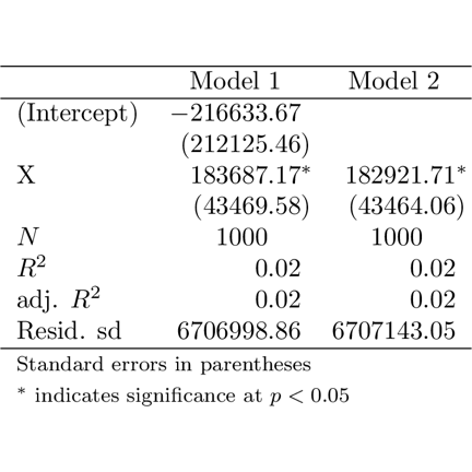

stargazer

require(stargazer)

## Loading required package: stargazer
## 
## Please cite as: 
## 
##  Hlavac, Marek (2013). stargazer: LaTeX code and ASCII text for well-formatted regression and summary statistics tables.
##  R package version 4.5.3. http://CRAN.R-project.org/package=stargazer

stargazer(dat.lm, dat.lm2)

## 
## % Table created by stargazer v.4.5.3 by Marek Hlavac, Harvard University. E-mail: hlavac at fas.harvard.edu
## % Date and time: Tue, Jan 28, 2014 - 23:38:48
## \begin{table}[!htbp] \centering 
##   \caption{} 
##   \label{} 
## \begin{tabular}{@{\extracolsep{5pt}}lcc} 
## \\[-1.8ex]\hline 
## \hline \\[-1.8ex] 
##  & \multicolumn{2}{c}{\textit{Dependent variable:}} \\ 
## \cline{2-3} 
## \\[-1.8ex] & \multicolumn{2}{c}{Y} \\ 
## \\[-1.8ex] & (1) & (2)\\ 
## \hline \\[-1.8ex] 
##  X & 183,687.000$^{***}$ & 182,922.000$^{***}$ \\ 
##   & (43,470.000) & (43,464.000) \\ 
##   & & \\ 
##  Constant & $-$216,634.000 &  \\ 
##   & (212,125.000) &  \\ 
##   & & \\ 
## \hline \\[-1.8ex] 
## Observations & 1,000 & 1,000 \\ 
## R$^{2}$ & 0.018 & 0.017 \\ 
## Adjusted R$^{2}$ & 0.017 & 0.016 \\ 
## Residual Std. Error & 6,706,999.000 (df = 998) & 6,707,143.000 (df = 999) \\ 
## F Statistic & 17.860$^{***}$ (df = 1; 998) & 17.710$^{***}$ (df = 1; 999) \\ 
## \hline 
## \hline \\[-1.8ex] 
## \textit{Note:}  & \multicolumn{2}{r}{$^{*}$p$<$0.1; $^{**}$p$<$0.05; $^{***}$p$<$0.01} \\ 
## \normalsize 
## \end{tabular} 
## \end{table}

stargazer

img <- readPNG("stargazer.png")
grid.raster(img)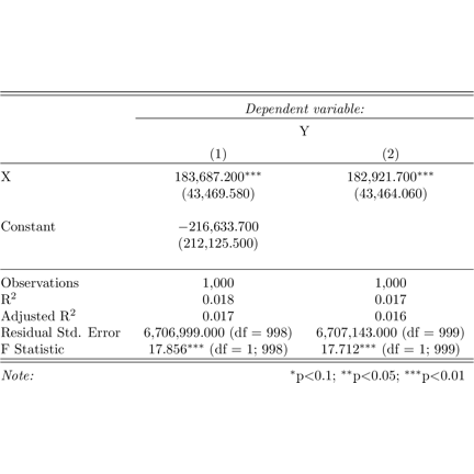

Both

Both packages are good (and can be supplemented with xtable when it is easier)
Get pretty close to what you want with these packages, and then tweak the LaTeX directly.

Plotting

It’s all about coordinate pairs.
plot(x,y) plots the pairs of points in x and y
Notable options:
- type - determines whether you plot points, lines or whatnot
- pch - determines plotting character
- xlim - x limits of the plot (likewise for y)
- xlab - label on the x-axis
- main - main plot label
- col - color
- A massive number of options. Read the docs.
Some objects respond specially to plot. Try plot(dat.lm)

Tying it Together

x <- seq(-1, 1, 0.01)
y <- 3/4 * (1 - x^2)
plot(x, y, type = "l", xlab = "h", ylab = "weight")

Tying it Together

\(W\) is an \(n\times p\) diagonal weighting matrix, \(h\) is a “bandwidth”.
Diagonal entries are \(\frac{3}{4}\cdot(1-d^2)\cdot 1_{\{|d|\le 1\}}\) where \(d = \frac{X-c}{h}\)
\(\hat{\beta}_c = (X'WX)^{-1}X'WY\)
Covariance matrix is \(s^2(X'WX)^{-1}\)

loc.lin <- function(Y, X, c = 0, bw = sd(X)/2) {
    d <- (X - c)/bw
    W <- 3/4 * (1 - d^2) * (abs(d) < 1)
    W <- diag(W)
    X <- cbind(1, d)
    b <- solve(t(X) %*% W %*% X) %*% t(X) %*% W %*% Y
    sigma <- t(Y - X %*% b) %*% W %*% (Y - X %*% b)/(sum(diag(W) > 0) - 2)
    sigma <- solve(t(X) %*% W %*% X) * c(sigma)
    return(c(est = b[1], se = sqrt(diag(sigma))[1]))
}

Fit the Surface

X.est <- seq(0, 5, 0.1)
dat.llm <- sapply(X.est, function(x) loc.lin(Y, X, c = x, bw = 0.25))
plot(X, Y, xlim = c(0, 5), ylim = c(-50, 50), pch = 20)
lines(X.est, dat.llm[1, ], col = "red")
lines(X.est, dat.llm[1, ] + 1.96 * dat.llm[2, ], col = "pink")
lines(X.est, dat.llm[1, ] - 1.96 * dat.llm[2, ], col = "pink")

Quant II Recitation

January 30, 2015

What is this?

Today’s Topic

Sharing

Workflow

When things break

Resources

Reading R Documentation

CRAN documentation

JSS

Confusing Things

Using Third-party Code

Data types

Character

Numeric

Logical

Objects

Data Structures

Vectors

Vectors (cont.)

More Vectors

Missingness

Lists

Matrices

Matrix Operations

More Matrix Ops.

Naming Things

Dataframes

Control Flow

Loops

If/Else

Vectorized If/Else

Functions

Useful Functions

Distributional Functions

Robust SEs

Multiple Dispactch

The *apply family

apply

sapply

tapply

Working With Data

Input

Simulate some Data

Regression Output

Regression Output

Pretty Output

xtable

xtable

Pretty it up

apsrtable

apsrtable

stargazer

stargazer

Both

Plotting

Tying it Together

Tying it Together

Fit the Surface