Structure of Class

• Today we're going to talk about:
  1. *apply functions
  2. Marginal Effects
  3. Sensitivity analysis for post-treament bias

The *apply family

• These functions allow one to efficiently perform a large number of actions on data.
• apply - performs actions on the rows or columns of a matrix/array (1 for rows, 2 for columns, 3 for ??)
• sapply - performs actions on every element of a vector
• tapply - performs actions on a vector by group
• replicate - performs the same action a given number of times

apply

A

##   c d
## a 1 3
## b 2 4

apply(A, 1, sum)

## a b 
## 4 6

apply(A, 2, mean)

##   c   d 
## 1.5 3.5

sapply

vec

## [1] "a" "b" "c"

sapply(vec, function(x) paste0(x, ".vec"))

##       a       b       c 
## "a.vec" "b.vec" "c.vec"

• Can be accomplished more simply with:

paste0(vec, ".vec")

## [1] "a.vec" "b.vec" "c.vec"

tapply

tapply(1:10, makeGroups(5, 2), mean)

##   1   2   3   4   5 
## 1.5 3.5 5.5 7.5 9.5

Local Linear Regression

• \(W\) is an \(n\times p\) diagonal weighting matrix, \(h\) is a "bandwidth".
• Diagonal entries are \(\frac{3}{4}\cdot(1-d^2)\cdot 1_{\{|d|\le 1\}}\) where \(d = \frac{X-c}{h}\)
• \(\hat{\beta}_c = (X'WX)^{-1}X'WY\)
• Covariance matrix is \(s^2(X'WX)^{-1}\)

loc.lin <- function(Y, X, c = 0, bw = sd(X)/2) {
    d <- (X - c)/bw
    W <- 3/4 * (1 - d^2) * (abs(d) < 1)
    W <- diag(W)
    X <- cbind(1, d)
    b <- solve(t(X) %*% W %*% X) %*% t(X) %*% W %*% Y
    sigma <- t(Y - X %*% b) %*% W %*% (Y - X %*% b)/(sum(diag(W) > 0) - 2)
    sigma <- solve(t(X) %*% W %*% X) * c(sigma)
    return(c(est = b[1], se = sqrt(diag(sigma))[1]))
}

Simulate some Data

set.seed(1023)  # Important for replication
X <- rnorm(1000, 0, 5)
Y <- sin(5 * X) * exp(abs(X)) + rnorm(1000)
dat <- data.frame(X, Y)
plot(X, Y, xlim = c(0, 5), ylim = c(-50, 50))

Look at the Kernel

x <- seq(-1, 1, 0.01)
y <- 3/4 * (1 - x^2)
plot(x, y, type = "l", xlab = "h", ylab = "weight")

Fit the Surface

X.est <- seq(0, 5, 0.1)
dat.llm <- sapply(X.est, function(x) loc.lin(Y, X, c = x, bw = 0.25))
plot(X, Y, xlim = c(0, 5), ylim = c(-50, 50), pch = 20)
lines(X.est, dat.llm[1, ], col = "red")
lines(X.est, dat.llm[1, ] + 1.96 * dat.llm[2, ], col = "pink")
lines(X.est, dat.llm[1, ] - 1.96 * dat.llm[2, ], col = "pink")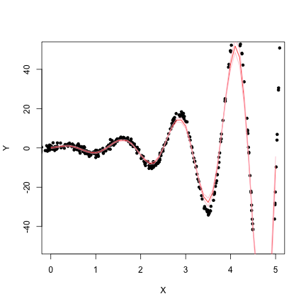

Introduce Example

• We'll be working with data from a paper in the most recent issue of IO.
• Helfer, L.R. and E. Voeten. (2014) "International Courts as Agents of Legal Change: Evidence from LGBT Rights in Europe"
• The treatment we are interested in is the presence of absence of a ECtHR judgment.
• The outcome is the adoption of progressive LGBT policy.
• And there's a battery of controls, of course.
• Voeten has helpfully put all replication materials online.

Prepare example

require(foreign, quietly = TRUE)
d <- read.dta("replicationdataIOLGBT.dta")
# Base specification
d$ecthrpos <- as.double(d$ecthrpos) - 1
d.lm <- lm(policy ~ ecthrpos + pubsupport + ecthrcountry + lgbtlaws + cond + 
    eumember0 + euemploy + coemembe + lngdp + year + issue + ccode, d)
d <- d[-d.lm$na.action, ]
d$issue <- as.factor(d$issue)
d$ccode <- as.factor(d$ccode)
summary(d.lm)$coefficients[1:11, ]

##                Estimate Std. Error t value  Pr(>|t|)
## (Intercept)  -1.589e+00  4.956e-01 -3.2052 1.360e-03
## ecthrpos      6.501e-02  1.056e-02  6.1537 8.289e-10
## pubsupport    6.549e-03  2.743e-03  2.3877 1.700e-02
## ecthrcountry  1.297e-01  3.584e-02  3.6201 2.980e-04
## lgbtlaws      2.358e-02  6.281e-03  3.7548 1.759e-04
## cond          9.277e-02  1.796e-02  5.1657 2.509e-07
## eumember0    -8.586e-03  8.498e-03 -1.0105 3.123e-01
## euemploy      3.659e-03  1.269e-02  0.2883 7.731e-01
## coemembe      2.083e-02  7.277e-03  2.8623 4.227e-03
## lngdp        -7.522e-07  4.501e-07 -1.6711 9.477e-02
## year          8.020e-04  2.522e-04  3.1799 1.484e-03

Marginal Effects

• There has seemed to be a bit of confusion over marginal effects.
• The Blattman paper in HW3 uses marginal effects "well" in the sense of causal inference.
• The Huber et al. paper uses them in a very standard way, but perhaps not the way we'd want to think about them in THIS class.
• Use the builtin predict function; it will make your life easier.

d.lm.interact <- lm(policy ~ ecthrpos * pubsupport + ecthrcountry + lgbtlaws + 
    cond + eumember0 + euemploy + coemembe + lngdp + year + issue + ccode, d)
frame0 <- frame1 <- model.frame(d.lm.interact)
frame0[, "ecthrpos"] <- 0
frame1[, "ecthrpos"] <- 1
meff <- mean(predict(d.lm.interact, newd = frame1) - predict(d.lm.interact, 
    newd = frame0))
meff

## [1] 0.08197

Delta Method

• Note 1: We know that our vector of coefficients are asymptotically multivariate normal.
• Note 2: We can approximate the distribution of many (not just linear) functions of these coefficients using the delta method.
• Delta method says that you can approximate the distribution of \(h(b_n)\) with \(\bigtriangledown{h}(b)'\Omega\bigtriangledown{h}(b)\) Where \(\Omega\) is the asymptotic variance of \(b\).
• In practice, this means that we just need to be able to derive the function whose distribution we wish to approximate.

Trivial Example

• We're interested in the ratio of the coefficient on ecthrpos to that of pubsupport.
• Call it \(b_2 \over b_3\). The gradient is \((\frac{1}{b_3}, \frac{b_2}{b_3^2})\)
• Estimate this easily in R with:

grad <- c(1/coef(d.lm)[3], coef(d.lm)[2]/coef(d.lm)[3]^2)
grad

## pubsupport   ecthrpos 
##        334       8046

se <- sqrt(t(grad) %*% vcov(d.lm)[2:3, 2:3] %*% grad)
est <- coef(d.lm)[2]/coef(d.lm)[3]
c(estimate = est, std.error = se)

## estimate.ecthrpos         std.error 
##             24.09             35.33

require(car)
deltaMethod(d.lm, "ecthrpos/pubsupport")

##                     Estimate    SE
## ecthrpos/pubsupport    24.09 35.55

Linear Functions

• But for most "marginal effects", you don't need to use the delta method.
• Just remember your rules for variances.
• \(\text{var}(aX+bY) = a^2\text{var}(X) + b^2\text{var}(Y) + 2ab\text{cov}(X,Y)\)
• If you are just looking at changes with respect to a single variable, you can just multiply standard errors.
• That is, a change in a variable of 3 units means that the standard error for the marginal effect would be 3 times the standard error of the coefficient.
• This isn't what Clarify does, though. It is weird.

Zelig for Marginal Effects

• (Zelig works like Clarify. [gee, I wonder why?])

# install.packages('Zelig', repos='http://r.iq.harvard.edu', type='source')
require(Zelig, quietly = TRUE)
d.zg <- zelig(policy ~ ecthrpos * pubsupport + ecthrcountry + lgbtlaws + cond + 
    eumember0 + euemploy + coemembe + lngdp + year + issue + ccode, d, model = "ls", 
    cite = FALSE)
x0 <- setx(d.zg, ecthrpos = 0)
x1 <- setx(d.zg, ecthrpos = 1)
out <- sim(d.zg, x = x0, x1 = x1)
c(mean(out$qi$fd), meff)

## [1] 0.08150 0.08197

Sensitivity Analysis

• We're adding to Cyrus's discussion on post-treatment bias with a sensitivity analysis.
• This is also in Rosenbaum (1984), which he mentioned in class.
• The variable which one might think could induce post-treatment bias in our example is that of "public acceptance".

Rosenbaum Bounding

• In general Rosenbaum is a proponent of trying to "bound" biases.
• He does this in his "normal" sensitivity analysis method, and we do the same, here.
• We will assume a "surrogate" for \(U\) (necessary for CIA), which is observed post-treatment.
• The surrogate has two potential outcomes: \(S_1\) and \(S_0\)
• It is presumed to have a linear response on the outcome.
• (As are the other observed covariates)
• This gives us the following two regression models: \(E[Y_1|S_1 = s , X = x] = \mu_1 + \beta' x + \gamma's\) and
  \(E[Y_0|S_0 = s , X = x] = \mu_0 + \beta' x + \gamma's\)
• This gives us:
  \(\tau = E[ (\mu_1 + \beta' X + \gamma'S_1) - (\mu_0 + \beta' X + \gamma'S_0)]\)
• Which is equal to the following useful expression:
  \(\tau = \mu_1 - \mu_0 + \gamma'( E[S_1 - S_0])\)
• For us, this means that \(\tau = \beta_1 + \beta_2 E[S_1 - S_0]\)

Back to example

• Our surrogate is public acceptance.
• But it can be swayed by court opinions, right? This is at least plausible.
• Let's try and get some reasonable bounds on \(\tau\).

sdS <- sd(d$pubsupport)
Ediff <- c(-1.5 * sdS, -sdS, -sdS/2, 0, sdS/2, sdS, 1.5 * sdS)
tau <- coef(d.lm)[2] + coef(d.lm)[3] * Ediff
names(tau) <- c("-1.5", "-1", "-.5", "0", ".5", "1", "1.5")
tau

##    -1.5      -1     -.5       0      .5       1     1.5 
## 0.06621 0.06818 0.07015 0.07212 0.07409 0.07606 0.07803