Regression Discontinuity
Drew Dimmery
April 4, 2014
Structure
- RDD interpretation
- RDD estimation
- Placebo tests
- Sorting
- Other stuff
Interpretation
- It's a LATE!
- A different kind of LATE!
- It can be interpreted as a weighted average over all units (Lee & Lemieux 2010)
- \((W,U)\) are observed and unobserved factors which explain all heterogeneity.
- \(X=c\) is the cutpoint on the running variable, \(Y\) is the outcome \(\lim_{\epsilon \downarrow 0} E[Y|X=c+\epsilon] - \lim_{\epsilon\uparrow 0} E[Y|X=c+\epsilon]\)
\(= \sum_{w,u} \tau(w,u) p(W=w,U=u|X=c)\)
\(= \sum_{w,u} \tau(w,u) {f(c|W=w,U=u) \over f(c)} p(W=w,U=u)\) - What does this mean?
- It's a weight of individual treatment effects weighted by the likelihood that a unit will lie near the threshhold on the running variable.
- Keep this in mind as you interpret results.
Estimation
- If only someone wrote a package to do this...
- http://github.com/ddimmery/rdd
- The current best pracices is to use local polynomial regression.
- Typically linear
- There are also some interesting methods using randomization inference, though. (Cattaneo et al n.d.)
Replication
- I'll be replicating the recent Meyersson paper that's been making noise.
- Replication materials
- The paper shows a (local) result that when Islamic parties won elections in Turkey, this resulted in better outcomes for women.
- Running variable: vote margin (but not exclusively 2 party system as in Lee)
- Outcome that we'll look at: high school education
require(foreign, quietly = TRUE)
d <- read.dta("regdata0.dta")
summary(d$iwm94)
## Min. 1st Qu. Median Mean 3rd Qu. Max. NA's
## -1.0 -0.5 -0.3 -0.3 -0.1 1.0 544Explore data
- Plot the raw data.
with(d, plot(iwm94, hischshr1520f, pch = 19, cex = 0.2, xlim = c(-0.5, 0.5)))
left.lm <- lm(hischshr1520f ~ iwm94, d, subset = iwm94 < 0)
right.lm <- lm(hischshr1520f ~ iwm94, d, subset = iwm94 >= 0)
left.x <- seq(-0.5, 0, 0.01)
right.x <- -left.x
lines(left.x, predict(left.lm, newd = data.frame(iwm94 = left.x)), col = "red")
lines(right.x, predict(right.lm, newd = data.frame(iwm94 = right.x)), col = "red")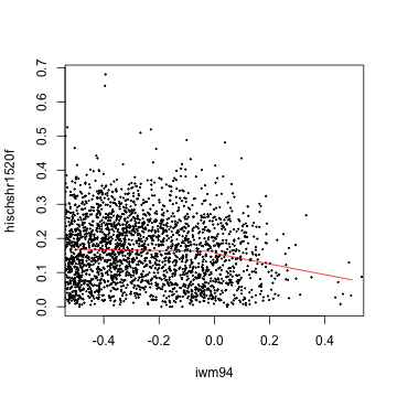
Estimation
- So the basic estimation would just take the difference of the intercepts from
left.lmandright.lm. - And there's an equivalency to just running a single regression as Cyrus showed in class.
- But I'm just going to use
rdd
require(rdd, quietly = TRUE)## Loading required package: zoo
##
## Attaching package: 'zoo'
##
## The following objects are masked from 'package:base':
##
## as.Date, as.Date.numeric
##
## Loading required package: car
## Loading required package: survival
## Loading required package: splinesrd.out <- RDestimate(hischshr1520f ~ iwm94, d)
rd.out##
## Call:
## RDestimate(formula = hischshr1520f ~ iwm94, data = d)
##
## Coefficients:
## LATE Half-BW Double-BW
## 0.0296 0.0250 0.0228Full Results
summary(rd.out)##
## Call:
## RDestimate(formula = hischshr1520f ~ iwm94, data = d)
##
## Type:
## sharp
##
## Estimates:
## Bandwidth Observations Estimate Std. Error z value
## LATE 0.24 1020 0.0296 0.0124 2.39
## Half-BW 0.12 589 0.0250 0.0165 1.52
## Double-BW 0.48 2050 0.0228 0.0101 2.26
## Pr(>|z|)
## LATE 0.0169 *
## Half-BW 0.1286
## Double-BW 0.0240 *
## ---
## Signif. codes: 0 '***' 0.001 '**' 0.01 '*' 0.05 '.' 0.1 ' ' 1
##
## F-statistics:
## F Num. DoF Denom. DoF p
## LATE 4.99 3 1016 3.86e-03
## Half-BW 1.70 3 585 3.30e-01
## Double-BW 25.77 3 2046 4.44e-16Plot it
plot(rd.out, range = c(-0.4, 0.4))
title(xlab = "Islamic Party Vote Margin", ylab = "Female High School Education Share")
Placebo tests
- Do placebo tests on other covariates and other outcomes.
- They're "placebo" because there "shouldn't" be an effect on them (except occasionally by chance)
# Age 19+
RDestimate(ageshr19 ~ iwm94, d)[c("est", "se")]
## $est
## LATE Half-BW Double-BW
## -0.003737 0.006946 -0.004117
##
## $se
## [1] 0.010314 0.013783 0.008307# Log Population
RDestimate(lpop1994 ~ iwm94, d)[c("est", "se")]## $est
## LATE Half-BW Double-BW
## 0.06921 -0.04339 0.03000
##
## $se
## [1] 0.2384 0.3276 0.1879# Household Size
RDestimate(shhs ~ iwm94, d)[c("est", "se")]## $est
## LATE Half-BW Double-BW
## -0.006963 0.321148 -0.091759
##
## $se
## [1] 0.3543 0.5431 0.2557More Placebos
# Men in 2000
RDestimate(hischshr1520m ~ iwm94, d)[c("est", "se")]
## $est
## LATE Half-BW Double-BW
## 0.009632 0.016188 0.007619
##
## $se
## [1] 0.009037 0.011807 0.007435# Women in 1990 (pre-treatment)
RDestimate(c90hischshr1520f ~ iwm94, d)[c("est", "se")]## $est
## LATE Half-BW Double-BW
## 0.0079389 0.0007974 0.0130517
##
## $se
## [1] 0.012239 0.017631 0.009308# Men in 1990 (pre-treatment)
RDestimate(c90hischshr1520m ~ iwm94, d)[c("est", "se")]## $est
## LATE Half-BW Double-BW
## 0.005930 0.002779 0.003861
##
## $se
## [1] 0.009770 0.013259 0.007891Sorting
- As Cyrus discussed, density tests are also a good way to examine the possibility of sorting.
DCdensity(d$iwm94, verbose = TRUE, plot = FALSE)## Assuming cutpoint of zero.
## Using calculated bin size: 0.009
## Using calculated bandwidth: 0.165
## Log difference in heights is -0.095 with SE 0.147
## this gives a z-stat of -0.650
## and a p value of 0.515## [1] 0.5154Density Plot
DCdensity(d$iwm94)
## [1] 0.5154Fuzzy designs
- I don't have an example for this, but it's quite easy.
- Do it the same way as before, but with
RDestimate(Y~runvar+treatment)
Overall
- Some big things for RDD:
- Lots of plots
- Think about locality in interpretation
- Use your covariates for robustness/placebo tests
- Everything should be robust to different bandwidths, etc
- If effects start disappearing as bw goes down, that's a bad sign.
- Your bandwidth is probably to wide.
- If there's still more time, maybe I'll go through some high points of the
rddcode.