Heterogeneity

Drew Dimmery

April 10, 2014

Structure

Define heterogeneity
Why I hate marginal effect plots
How to do it "right"

Definition

We are interested in the causal effect of \(D\) on \(Y\) at \(X=x\):
\(E[Y_1 - Y_0 | X=x]\)
This is not a "causal difference"
It can reflect selection of units to particular \(x\), etc

Simulation

x <- runif(100)
x <- c(x, abs(rnorm(100)))
d <- rbinom(200, 1, 0.5)
y0 <- rnorm(200, 0, 0.25)
y1 <- 3 + 2 * cos(2 * x) + rnorm(200, 0, 0.25)
tau <- mean(y1 - y0)
y <- y1 * d + y0 * (1 - d)
simple <- lm(y ~ d)
interact <- lm(y ~ d + d * x)
c(tau, coef(simple)["d"], coef(interact)["d"] + coef(interact)["d:x"] * mean(x))

##           d     d 
## 3.560 3.655 3.570

Plot simulation

plot(x,y0,pch="0",cex=.5,ylim=c(min(c(y0,y1)),max(c(y0,y1))),ylab="y")
points(x,y1,pch="1",cex=.5)
x.fit <- seq(min(x),max(x),.01)
n.fit <- length(x.fit)
fit.true <- 3+2*cos(2*x.fit)
lines(x.fit,fit.true,lty="dotted",col="red")
lines(x.fit,rep(0,n.fit),lty="dotted",col="red")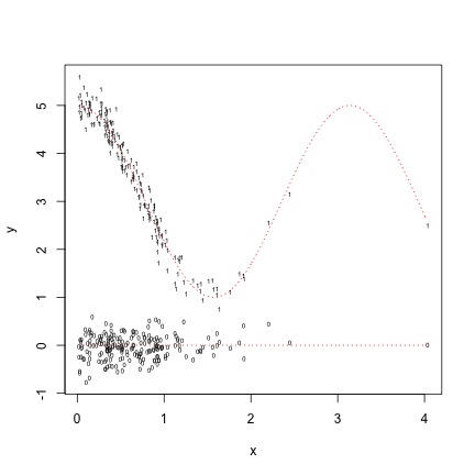

Marginal Effects

plot(x.fit, rep(tau, n.fit), col = "black", type = "l", xlab = "x", ylab = "TE", 
    ylim = c(1, 5))
lines(x.fit, fit.true, col = "black", lty = "twodash")
rug(x)
simple.pred <- diff(predict(simple, newd = data.frame(d = c(0, 1))))
simple.se <- sqrt(var(y[d == 1])/sum(d == 1) + var(y[d == 0])/sum(d == 0))
simple.upr <- simple.pred + 1.96 * simple.se
simple.lwr <- simple.pred - 1.96 * simple.se
lines(x.fit, rep(simple.pred, n.fit), col = "blue")
lines(x.fit, rep(simple.upr, n.fit), col = "blue", lty = "dotted")
lines(x.fit, rep(simple.lwr, n.fit), col = "blue", lty = "dotted")
x.fit.frame <- data.frame(d = c(rep(1, n.fit), rep(0, n.fit)), x = rep(x.fit, 
    2))
interact.pred <- predict(interact, newd = x.fit.frame)
interact.pred <- interact.pred[1:n.fit] - interact.pred[{
    n.fit + 1
}:{
    2 * n.fit
}]
vcv.int <- vcov(interact)
interact.se.model <- sqrt(vcv.int["d", "d"] + x.fit^2 * vcv.int["d:x", "d:x"] + 
    2 * x.fit * vcv.int["d", "d:x"])
interact.upr <- interact.pred + 1.96 * interact.se.model
interact.lwr <- interact.pred - 1.96 * interact.se.model
lines(x.fit, interact.pred, col = "red")
lines(x.fit, interact.upr, col = "red", lty = "dotted")
lines(x.fit, interact.lwr, col = "red", lty = "dotted")
legend("topright", legend = c("Tau", "Tau(x)", "Simple TE est", "Interacted TE est"), 
    lty = c("solid", "twodash", "solid", "solid"), col = c("black", "black", 
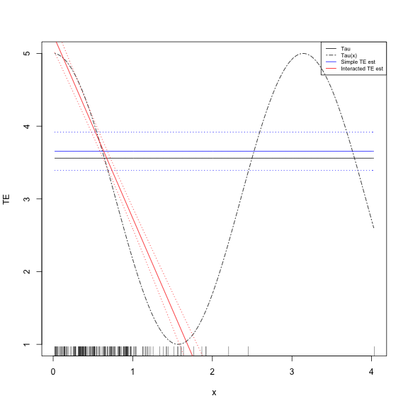
        "blue", "red"), cex = 0.65)

Show the plot

One of the most dangerous plots in social science:

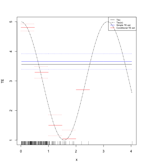
What instead?

One possibility is to plot estimates in strata.
This will actually preserve your "true" uncertainty in certain areas.

strata <- cbind(lwr = c(0, 0.5, 1, 1.5, 2, 2.5), upr = c(0.5, 1, 1.5, 2, 2.5, 
    3))
getTE <- function(z) {
    lwr <- z[1]
    upr <- z[2]
    in.strata <- x >= lwr & x < upr
    N1 <- sum(in.strata & d == 1)
    N0 <- sum(in.strata & d == 0)
    if (N1 < 1 | N0 < 1) 
        return(c(te = NA, upr = NA, lwr = NA))
    mod <- lm(y ~ d, subset = in.strata)
    se <- sqrt(var(y[in.strata & d == 1])/N1 + var(y[in.strata & d == 0])/N0)
    te <- diff(predict(mod, newd = data.frame(d = c(0, 1))))
    upr <- te + 1.96 * se
    lwr <- te - 1.96 * se
    names(te) <- names(upr) <- names(lwr) <- NULL
    return(c(te = te, upr = upr, lwr = lwr))
}
TEs <- apply(strata, 1, getTE)

Plot Stratum Effects

plot(x.fit, rep(tau, n.fit), col = "black", type = "l", xlab = "x", ylab = "TE", 
    ylim = c(1, 5))
lines(x.fit, fit.true, col = "black", lty = "twodash")
rug(x)
lines(x.fit, rep(simple.pred, n.fit), col = "blue")
lines(x.fit, rep(simple.upr, n.fit), col = "blue", lty = "dotted")
lines(x.fit, rep(simple.lwr, n.fit), col = "blue", lty = "dotted")
for (i in 1:nrow(strata)) {
    x.fit.strata <- seq(strata[i, 1], strata[i, 2], 0.01)
    n.fit.strata <- length(x.fit.strata)
    lines(x.fit.strata, rep(TEs["te", i], n.fit.strata), col = "red")
    lines(x.fit.strata, rep(TEs["lwr", i], n.fit.strata), col = "red", lty = "dotted")
    lines(x.fit.strata, rep(TEs["upr", i], n.fit.strata), col = "red", lty = "dotted")
}
legend("topright", legend = c("Tau", "Tau(x)", "Simple TE est", "Conditional TE est"), 
    lty = c("solid", "twodash", "solid", "solid"), col = c("black", "black", 
        "blue", "red"), cex = 0.65)

And the plot

Generalize that a little

y1.fit <- predict(loess(y ~ x, subset = d == 1), newd = data.frame(x = x.fit), 
    se = TRUE)
y0.fit <- predict(loess(y ~ x, subset = d == 0), newd = data.frame(x = x.fit), 
    se = TRUE)
TE.pred <- y1.fit$fit - y0.fit$fit
SE.pred <- sqrt(y1.fit$se^2 + y0.fit$se^2)
TE.upr <- TE.pred + 1.96 * SE.pred
TE.lwr <- TE.pred - 1.96 * SE.pred
plot(x.fit, rep(tau, n.fit), col = "black", type = "l", xlab = "x", ylab = "TE", 
    ylim = c(1, 5))
lines(x.fit, fit.true, col = "black", lty = "twodash")
rug(x)
lines(x.fit, TE.pred, col = "red")
lines(x.fit, TE.upr, col = "red", lty = "dotted")
lines(x.fit, TE.lwr, col = "red", lty = "dotted")
legend("topright", legend = c("Tau", "Tau(x)", "LOESS TE est"), lty = c("solid", 
    "twodash", "solid"), col = c("black", "black", "red"), cex = 0.65)

And the plot

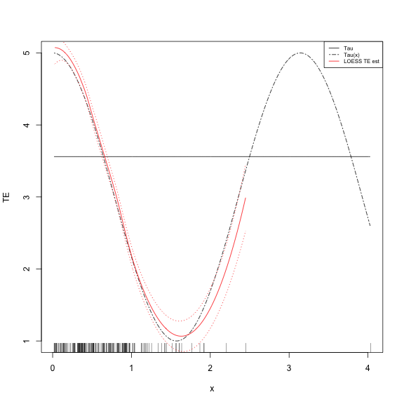
Why are the SEs so narrow in the area of sparsity?

Even better

Hill (2011)

require(BayesTree, quietly = TRUE)
bart.mod <- bart(cbind(d, x), y, rbind(cbind(1, x.fit), cbind(0, x.fit)), verbose = FALSE)
TE.pred <- bart.mod$yhat.test[, 1:n.fit] - bart.mod$yhat.test[, {
    n.fit + 1
}:{
    2 * n.fit
}]
TE.upr <- apply(TE.pred, 2, function(z) quantile(z, 0.975))
TE.lwr <- apply(TE.pred, 2, function(z) quantile(z, 0.025))
TE.pred <- colMeans(TE.pred)
plot(x.fit, rep(tau, n.fit), col = "black", type = "l", xlab = "x", ylab = "TE", 
    ylim = c(1, 5))
lines(x.fit, fit.true, col = "black", lty = "twodash")
rug(x)
lines(x.fit, TE.pred, col = "red")
lines(x.fit, TE.upr, col = "red", lty = "dotted")
lines(x.fit, TE.lwr, col = "red", lty = "dotted")
legend("topright", legend = c("Tau", "Tau(x)", "BART TE est"), lty = c("solid", 
    "twodash", "solid"), col = c("black", "black", "red"), cex = 0.65)

BART is Awesome

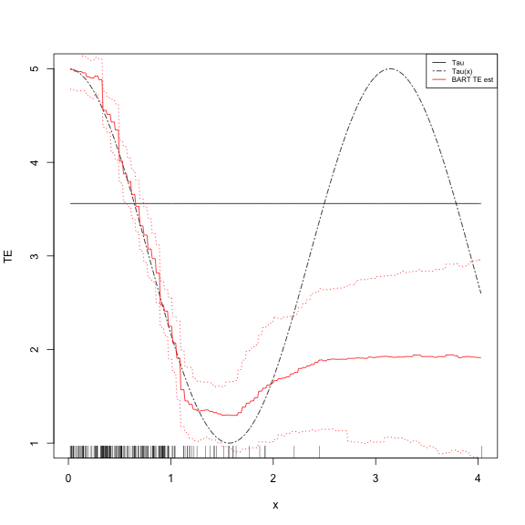
That represents our uncertainty quite well, doesn't it?

BART for ATE

Remember how Blattman calculated marginal effects?
What we do here is a sort of analogue to that procedure.
We marginalize our results from BART over the empirical distribution of \(x\).

bart.for.TE <- bart(cbind(d, x), y, rbind(cbind(1, x), cbind(0, x)), verbose = FALSE)
TE.pred <- bart.for.TE$yhat.test[, 1:200] - bart.for.TE$yhat.test[, {
    201
}:{
    400
}]
TE.pred <- rowMeans(TE.pred)
c(tau = tau, lwr = quantile(TE.pred, 0.025), TE = mean(TE.pred), upr = quantile(TE.pred, 
    0.975))

##       tau  lwr.2.5%        TE upr.97.5% 
##     3.560     3.518     3.588     3.659

Replication

"Are Voters More Likely to Contribute to Other Public Goods? Evidence from a Large-Scale Randomized Policy Experiment"
Bolsen, Ferraro and Miranda (2014) AJPS
Replication Materials
Outcome: Water use (reducing is "pro-social behavior")
Treatment: Appeals aimed at inducing pro-social behavior (and water use in particular)
Most relevant covariate is voting frequency

load("AJPS_ReplicationDataset.Rdata")
x$alltreat <- ifelse(x$treatment == 4, 0, 1)

full.mod <- lm(summer_07 ~ alltreat * perc_votecount_hh + unregistered + water_2006 + 
    apr_may_07 + fmv + y_max_yblt + owner + old + factor(route), x)
interact.mod <- lm(summer_07 ~ alltreat * perc_votecount_hh, x)
simple.mod <- lm(summer_07 ~ alltreat, x)
c(full = coef(full.mod)["alltreat"], interact = coef(interact.mod)["alltreat"] + 
    coef(interact.mod)["alltreat:perc_votecount_hh"] * mean(x$perc_votecount_hh, 
        na.rm = TRUE), simple = coef(simple.mod)["alltreat"])

##     full.alltreat interact.alltreat   simple.alltreat 
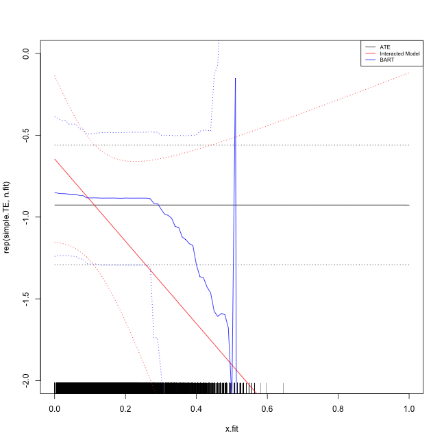
##           -0.6910           -0.9074           -0.9265

Examine Heterogeneity

We'll start with a simple difference in means as a benchmark, then develop a nice chart of the heterogeneity with respect to voting frequency.

simple.TE <- with(x, mean(summer_07[alltreat == 1]) - mean(summer_07[alltreat == 
    0]))
simple.SE <- with(x, sqrt(var(summer_07[alltreat == 1])/sum(alltreat == 1) + 
    var(summer_07[alltreat == 0])/sum(alltreat == 0)))
TE.upr <- simple.TE + 1.96 * simple.SE
TE.lwr <- simple.TE - 1.96 * simple.SE
x.fit <- seq(0, 1, 0.01)
n.fit <- length(x.fit)
plot(x.fit, rep(simple.TE, n.fit), ylim = c(-2, 0), type = "l")
rug(x$perc_votecount_hh)
lines(x.fit, rep(TE.upr, n.fit), lty = "dotted")
lines(x.fit, rep(TE.lwr, n.fit), lty = "dotted")
x.fit.frame <- data.frame(alltreat = c(rep(1, n.fit), rep(0, n.fit)), perc_votecount_hh = rep(x.fit, 
    2))
interact.pred <- predict(interact.mod, newd = x.fit.frame)
interact.pred <- interact.pred[1:n.fit] - interact.pred[{
    n.fit + 1
}:{
    2 * n.fit
}]
vcv.int <- vcov(interact.mod)
interact.se.model <- sqrt(vcv.int["alltreat", "alltreat"] + x.fit^2 * vcv.int["alltreat:perc_votecount_hh", 
    "alltreat:perc_votecount_hh"] + 2 * x.fit * vcv.int["alltreat", "alltreat:perc_votecount_hh"])
interact.upr <- interact.pred + 1.96 * interact.se.model
interact.lwr <- interact.pred - 1.96 * interact.se.model
lines(x.fit, interact.pred, col = "red")
lines(x.fit, interact.upr, col = "red", lty = "dotted")
lines(x.fit, interact.lwr, col = "red", lty = "dotted")

BART for heterogeneity

x.train <- cbind(x$alltreat, x$perc_votecount_hh)
y.train <- x$summer_07
ok <- complete.cases(x.train)
x.train <- x.train[ok, ]
y.train <- y.train[ok]
bart.int.mod <- bart(x.train, y.train, rbind(cbind(1, x.fit), cbind(0, x.fit)), 
    verbose = FALSE)
bart.pred <- bart.int.mod$yhat.test[, 1:n.fit] - bart.int.mod$yhat.test[, {
    n.fit + 1
}:{
    2 * n.fit
}]
bart.upr <- apply(bart.pred, 2, function(z) quantile(z, 0.975))
bart.lwr <- apply(bart.pred, 2, function(z) quantile(z, 0.025))
bart.pred <- colMeans(bart.pred)
lines(x.fit, bart.pred, col = "blue")
lines(x.fit, bart.upr, col = "blue", lty = "dotted")
lines(x.fit, bart.lwr, col = "blue", lty = "dotted")
legend("topright", legend = c("ATE", "Interacted Model", "BART"), lty = c("solid", 
    "solid", "solid"), col = c("black", "red", "blue"), cex = 0.65)

The final plot