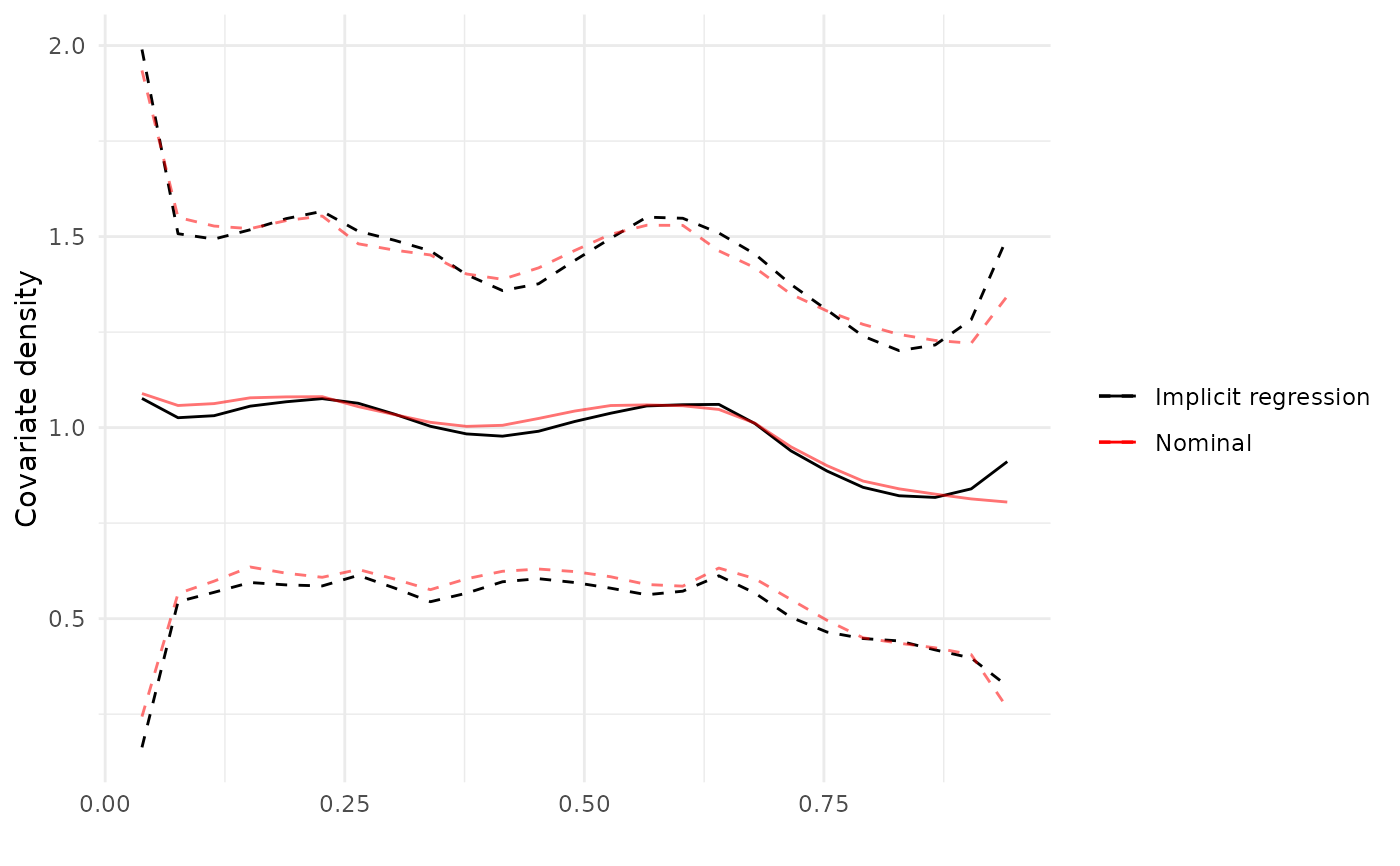
This provides a simple plot for the distribution of a single continuous covariate in the nominal sample and the implicit sample defined by the Aronow and Samii (2015) doi:10.1111/ajps.12185 regression weights.
plot_weighting_continuous(mod, covariate, alpha = 0.05, num_eval = 250, ...)Arguments
Value
A ggplot2::ggplot object.
Details
Kernel density estimates use the bias-corrected methods of Cattaneo et al (2020).
References
Cattaneo, Jansson and Ma (2021): lpdensity: Local Polynomial Density Estimation and Inference. Journal of Statistical Software, forthcoming.
Cattaneo, Jansson and Ma (2020): Simple Local Polynomial Density Estimators. Journal of the American Statistical Association 115(531): 1449-1455.