Example Usage

Introduction

Aronow and Samii (2015) provide a convenient way to understand why a linear regression provides the particular estimate that it does. Given the following linear model estimated by OLS,

\[ Y = \alpha + \tau A + \beta \boldsymbol{X} \]

In the presence of heterogeneity in the effect of \(A\) on \(Y\), however, \(\hat{\tau}\) will be a weighted average of the unit-specific effects, \(\tau_i\):

\[ \frac{\mathbb{E}[w_i \tau_i]}{\mathbb{E}[w_i]}\quad \mathrm{where}\; w_i = (A_i - \mathbb{E}[A_i \mid X_i])^2 \]

This weight is equal to the conditional variance of \(A\) in expectation: \(\mathbb{E}[w_i \mid X_i] = \mathrm{var}(A_i \mid X_i)\).

These weights can be easily estimated through a partial linear regression of the form:

\[ A = \gamma \boldsymbol{X} \]

Implicit regression weights are then just the squared residuals of this regression.

The intuition of this is that a unit-specific coefficient in OLS will, in general, be up-weighted when it’s harder to explain that variable’s value from the other covariates in the model. If a unit’s \(A_i\) is very easy to predict, then it will not figure prominently in the aggregate OLS estimate of the effect.

This is distinct from more conventional regression diagnostics like leverage, because those focus on how the entire vector of coefficients change. Most analysts, however, have specific hypotheses on specific coefficients, however, so the implicit regression weights demonstrate, essentially, the term-specific leverage.

Load packages and setup environment

library(dplyr)

## 
## Attaching package: 'dplyr'

## The following objects are masked from 'package:stats':
## 
##     filter, lag

## The following objects are masked from 'package:base':
## 
##     intersect, setdiff, setequal, union

library(ggplot2)
library(sf)

## Linking to GEOS 3.10.2, GDAL 3.4.1, PROJ 8.2.1; sf_use_s2() is TRUE

library(regweight)
data("LaLonde", package = "CBPS")

df <- dplyr::filter(
  LaLonde,
  (exper == 1 & treat == 1) | (exper == 0 & treat == 0)
)

model <- lm(
  log(re78 + 1) ~ treat + age + educ + black + hisp + married + nodegr + log(re74 + 1) + log(re75 + 1) + re74.miss, 
  df
)
summary(model)

## 
## Call:
## lm(formula = log(re78 + 1) ~ treat + age + educ + black + hisp + 
##     married + nodegr + log(re74 + 1) + log(re75 + 1) + re74.miss, 
##     data = df)
## 
## Residuals:
##      Min       1Q   Median       3Q      Max 
## -10.3859   0.0860   0.5236   0.9107   7.2818 
## 
## Coefficients:
##                Estimate Std. Error t value Pr(>|t|)    
## (Intercept)    3.302403   0.483647   6.828 1.05e-11 ***
## treat          0.359638   0.225490   1.595 0.110845    
## age           -0.019126   0.005447  -3.511 0.000453 ***
## educ           0.051214   0.026673   1.920 0.054952 .  
## black          0.021713   0.129822   0.167 0.867184    
## hisp           0.399143   0.273189   1.461 0.144114    
## married        0.357764   0.153319   2.333 0.019695 *  
## nodegr        -0.242343   0.172315  -1.406 0.159719    
## log(re74 + 1)  0.172411   0.025421   6.782 1.44e-11 ***
## log(re75 + 1)  0.430511   0.024304  17.713  < 2e-16 ***
## re74.miss     -0.615033   0.182580  -3.369 0.000766 ***
## ---
## Signif. codes:  0 '***' 0.001 '**' 0.01 '*' 0.05 '.' 0.1 ' ' 1
## 
## Residual standard error: 2.697 on 2776 degrees of freedom
## Multiple R-squared:  0.3546, Adjusted R-squared:  0.3523 
## F-statistic: 152.6 on 10 and 2776 DF,  p-value: < 2.2e-16

Examine regression weights

Plots will make a best effort to infer the appropriate type of a given covariate. If you aren’t happy with how they look, it’s simple enough to use the underlying functions called by the S3 method directly. They are:

rw_mod <- calculate_weights(model, "treat")
hist(rw_mod) + scale_x_continuous("Weight")

## Scale for x is already present.
## Adding another scale for x, which will replace the existing scale.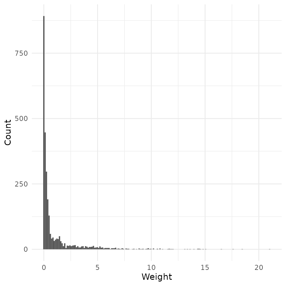

Discrete covariates

plot(rw_mod, df$married) + scale_x_continuous("Married", breaks = c(0, 1))

## Scale for x is already present.
## Adding another scale for x, which will replace the existing scale.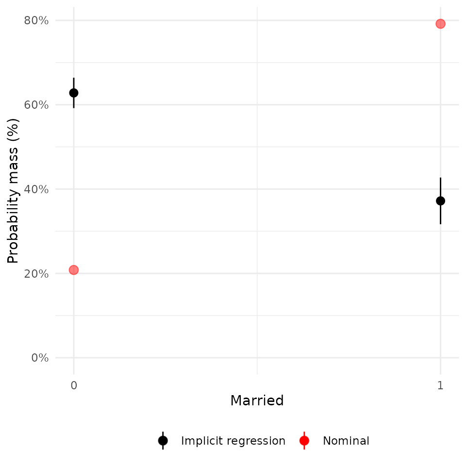

plot(rw_mod, df$nodegr) + scale_x_continuous("No degree", breaks = c(0, 1))

## Scale for x is already present.
## Adding another scale for x, which will replace the existing scale.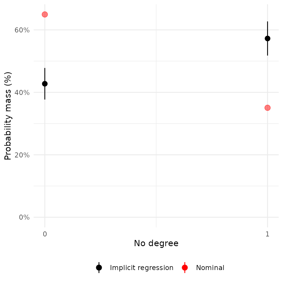

plot(rw_mod, df$black) + scale_x_continuous("Black", breaks = c(0, 1))

## Scale for x is already present.
## Adding another scale for x, which will replace the existing scale.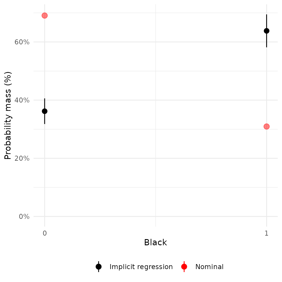

Continuous covariates

plot(rw_mod, df$age) + scale_x_continuous("Age")

## Scale for x is already present.
## Adding another scale for x, which will replace the existing scale.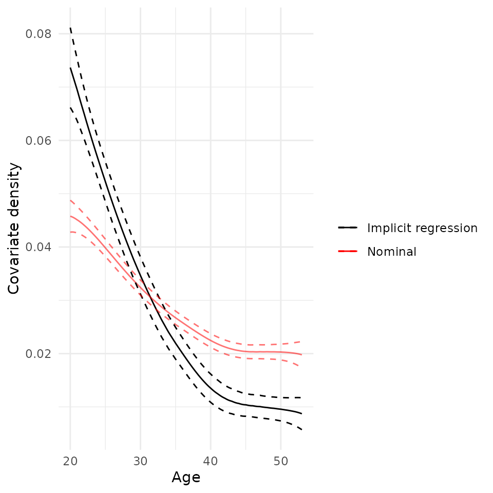

plot(rw_mod, df$re74) + scale_x_continuous("Income (1974)")

## Scale for x is already present.
## Adding another scale for x, which will replace the existing scale.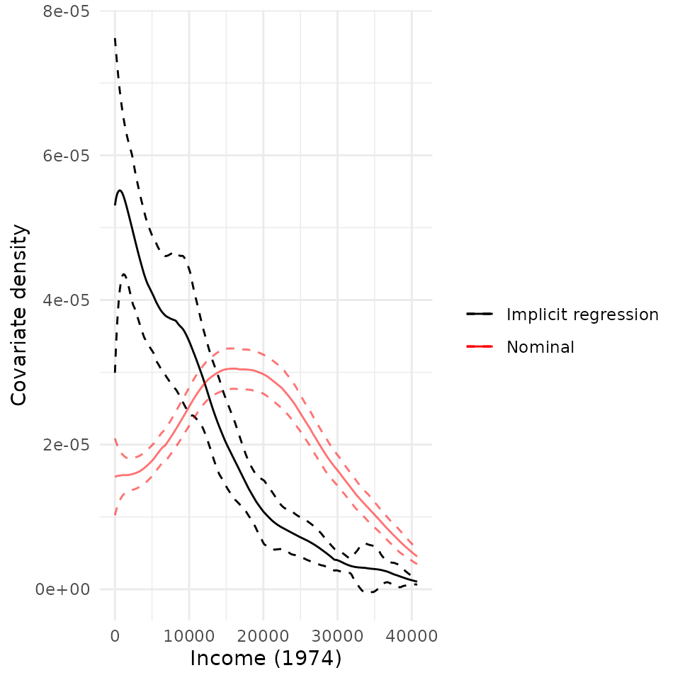

Summary table

It’s also easy to include a table of summary statistics for the nominal and implicit samples across a variety of covariates:

summary(
  rw_mod,
  df %>% select(re74, re74.miss, age, married, nodegr),
  output = "html"
)

Covariate	Value	Nominal		Implicit
Covariate	Value	Mean	Std. Dev.	Mean	Std. Dev.
Discrete variables
married	0	0.208		0.628
	1	0.792		0.372
nodegr	0	0.649		0.428
	1	0.351		0.572
re74.miss	0	0.901		0.959
	1	0.0994		0.0411
Continuous variables
age		33.8	10.6	28.5	9.59
re74		17,700	13,700	8,160	10,000

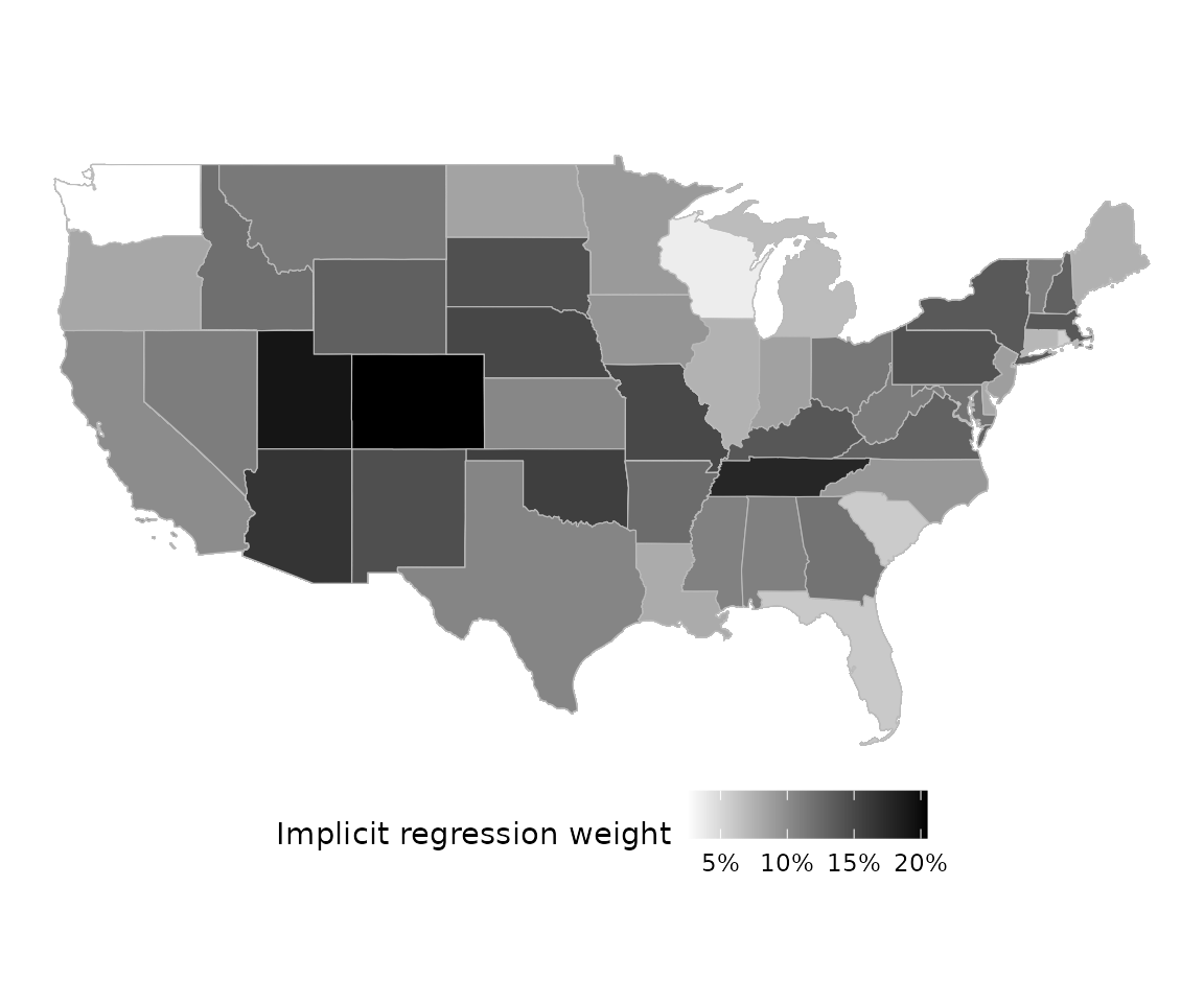
Mapping

For the sake of example, let’s imagine that we had geographical information on each unit, as well. Geometries/shapes should be specified in sf::sfc format.

state_shapes <- USAboundaries::us_states()
state_shapes <- dplyr::filter(state_shapes, !(state_abbr %in% c("HI", "PR", "AK")))
# Necessary due to https://github.com/r-spatial/sf/issues/1419
suppressWarnings(sf::st_crs(state_shapes) <- 4326)
pr_state <- seq(1, 10, length = nrow(state_shapes))
pr_state <- pr_state / sum(pr_state)
df$geometry <- sample(state_shapes$geometry, nrow(df), replace = TRUE, prob = pr_state)

plot(rw_mod, df$geometry)

Drew Dimmery (drew.dimmery@gmail.com)