HTE Analysis in an Experiment
Drew Dimmery (cran@ddimmery.com)
09 October, 2025
Source:vignettes/experimental_analysis.Rmd
experimental_analysis.RmdIntroduction
In this example analysis, I will demonstrate how to run an analysis of heterogeneous treatment effects in a randomized control trial using the methods of Kennedy (2023). This implies that propensity scores are known, so estimates will generally be unbiased.
This analysis will focus on using machine learning ensembles (through SuperLearner) to estimate nuisance functions and then provide a tibble of estimates of conditional treatment effects along with their associated standard errors.
Simulate data
If real data is used, simply replace this block with an appropriate
readr::read_csv call or equivalent, creating a tibble. I
will assume this tibble is stored as data for the remainder
of this document.
Note that datatypes can be either continuous or discrete, and that there can be columns in the tibble that are not included in any resulting anayses.
set.seed(100)
n <- 500
data <- tibble(
  uid = 1:n
) %>%
  mutate(
    a = rbinom(n, 1, 0.3),
    ps = rep(0.3, n),
    x1 = rnorm(n),
    x2 = factor(sample(1:4, n, prob = c(1 / 100, 39 / 100, 1 / 5, 2 / 5), replace = TRUE)),
    x3 = factor(sample(1:3, n, prob = c(1 / 5, 1 / 5, 3 / 5), replace = TRUE)),
    x4 = (x1 + rnorm(n)) / 2,
    x5 = rnorm(n),
    y = (
      a + x1 - a * (x1 - mean(x1)) + (4 * rbinom(n, 1, 0.5) - 1) * a * (x2 == 2) +
        a * (x2 == 3) + 0.5 * a * (x2 == 4) +
        0.25 * rnorm(n)
    ),
    w = 0.1 + rexp(n, 1 / 0.9)
  )
Define Recipe
Propensity Score Model
In this example, the propensity score is known because the data is from a randomized experiment. We don’t need to estimate a model for the propensity score.
For CATEs on discrete moderators, this implies that our estimates will simply be equivalent to AIPW estimators and will therefore inherit unbiasedness. For continuous moderators, similarly, if the CATE functions are smooth, we will attain consistency for recovering the true function non-parametrically.
Outcome Model
We estimate the outcome (T-learner) plugin estimate using an ensemble of machine learning models, including a wide array of model complexities from linear models, GAMs, regularized regressions. In this example, non-linear models are not included (due to runtime), but they could easily be added by uncommenting the associated lines.
Each individual component of the model provides a list of
hyperparameters, over which a full cross-product is taken and all
resulting models are estimate. For instance, SL.glmnet
sweeps over one hyperparameter (the mixing parameters between ridge and
Lasso). A model with each of the hyper-parameter values will be
estimated and incorporated into the ensemble. Note that
SL.glmnet automatically tunes the regularization parameter
using cv.glmnet, so this is not included as a
hyperparameter.
Quantities of interest
Quantities of Interest determine how results are reported to the user. You can think about this as determining, for instance how results should be plotted in a resulting chart.
For simplicity, this example simply provides results in one of two
ways: - Discrete covariates are stratified and the conditional effect is
plotted at each distinct level of the covariate. - Continuous covariates
have the effect surface estimated using local-linear regression via
nprobust of Calonico, Cattaneo and Farrell (2018). See,
similarly, Kennedy, Ma, McHugh and Small (2017) for justification of
this approach. Results are obtained for a grid of 100 quantiles across
the domain of the covariate.
An additional quantity of interest provided is the variable importance of a learned joint model of conditional effects (over all covariates). The approach implemented is described in Williamson, Gilbert, Carone and Simon (2020).
hte_cfg <- basic_config() %>%
  add_known_propensity_score("ps") %>%
  add_outcome_model("SL.glm.interaction") %>%
  add_outcome_model("SL.glmnet", alpha = c(0, 1)) %>%
  add_outcome_model("SL.glmnet.interaction", alpha = c(0, 1)) %>%
  add_outcome_diagnostic("RROC") %>%
  add_effect_model("SL.glm.interaction") %>%
  add_effect_model("SL.glmnet", alpha = c(0, 1)) %>%
  add_effect_model("SL.glmnet.interaction", alpha = c(0, 1)) %>%
  add_effect_diagnostic("RROC") %>%
  add_moderator("Stratified", x2, x3) %>%
  add_moderator("KernelSmooth", x1, x4, x5) %>%
  add_vimp(sample_splitting = FALSE)
## Super Learner## Version: 2.0-29## Package created on 2024-02-06Estimate Models
To actually perform the estimation, the following will be sufficient. Note that the configuration of covariate names at the top of the document makes all of this a little more complex with all the curly-brackets and bangs.
prepped_data <- data %>%
  attach_config(hte_cfg) %>%
  make_splits(uid, .num_splits = 3) %>%
  produce_plugin_estimates(
    y,
    a,
    x1, x2, x3, x4, x5,
  ) %>%
  construct_pseudo_outcomes(y, a)

results <- prepped_data %>%
  estimate_QoI(x1, x2, x3, x4, x5)
## Error in model.frame.default(Terms, newdata, na.action = na.action, xlev = object$xlevels) :
## factor x2 has new levels 1
## Error in model.frame.default(Terms, newdata, na.action = na.action, xlev = object$xlevels) :
## factor x2 has new levels 1
results## # A tibble: 839 × 6
## estimand term value level estimate std_error
## <chr> <chr> <dbl> <chr> <dbl> <dbl>
## 1 MCATE x1 -1.80 NA 3.22 0.173
## 2 MCATE x1 -1.71 NA 3.11 0.166
## 3 MCATE x1 -1.58 NA 2.96 0.157
## 4 MCATE x1 -1.47 NA 2.84 0.149
## 5 MCATE x1 -1.40 NA 2.78 0.145
## 6 MCATE x1 -1.35 NA 2.73 0.142
## 7 MCATE x1 -1.30 NA 2.69 0.139
## 8 MCATE x1 -1.26 NA 2.65 0.137
## 9 MCATE x1 -1.21 NA 2.60 0.135
## 10 MCATE x1 -1.16 NA 2.56 0.134
## # ℹ 829 more rowsATEs
## # A tibble: 1 × 6
##   estimand term  value level estimate std_error
##   <chr>    <chr> <dbl> <chr>    <dbl>     <dbl>
## 1 SATE     NA       NA NA        1.58     0.101
Plots
Plot Ensemble Coefficients
filter(results, grepl("SL coefficient", estimand)) %>%
  mutate(level = factor(level, levels = c("Control Response", "Treatment Response"))) %>%
  ggplot(aes(
    x = reorder(term, estimate),
    y = estimate,
    ymin = estimate - 1.96 * std_error,
    ymax = estimate + 1.96 * std_error
  )) +
  geom_abline(intercept = 0, slope = 0, linetype = "dashed") +
  geom_pointrange() +
  expand_limits(y = 0) +
  scale_x_discrete("Model name") +
  scale_y_continuous("Coefficient in SuperLearner Ensemble") +
  facet_wrap(~level) +
  coord_flip() +
  ggtitle("SuperLearner Ensemble") +
  theme_minimal()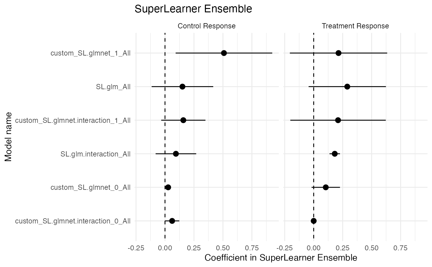
Plot risk for each submodel
filter(results, grepl("SL risk", estimand)) %>%
  mutate(
    level = factor(level, levels = c("Control Response", "Treatment Response", "Effect Surface"))
  ) %>%
  ggplot() +
  geom_abline(intercept = 0, slope = 0, linetype = "dashed") +
  geom_pointrange(aes(
    x = reorder(term, -estimate),
    y = estimate,
    ymin = estimate - 1.96 * std_error,
    ymax = estimate + 1.96 * std_error
  )) +
  expand_limits(y = 0) +
  scale_x_discrete("Model name") +
  scale_y_continuous("CV Risk in SuperLearner Ensemble") +
  facet_wrap(~level, scales = "free_x") +
  coord_flip() +
  ggtitle("Submodel Risk Estimates") +
  theme_minimal()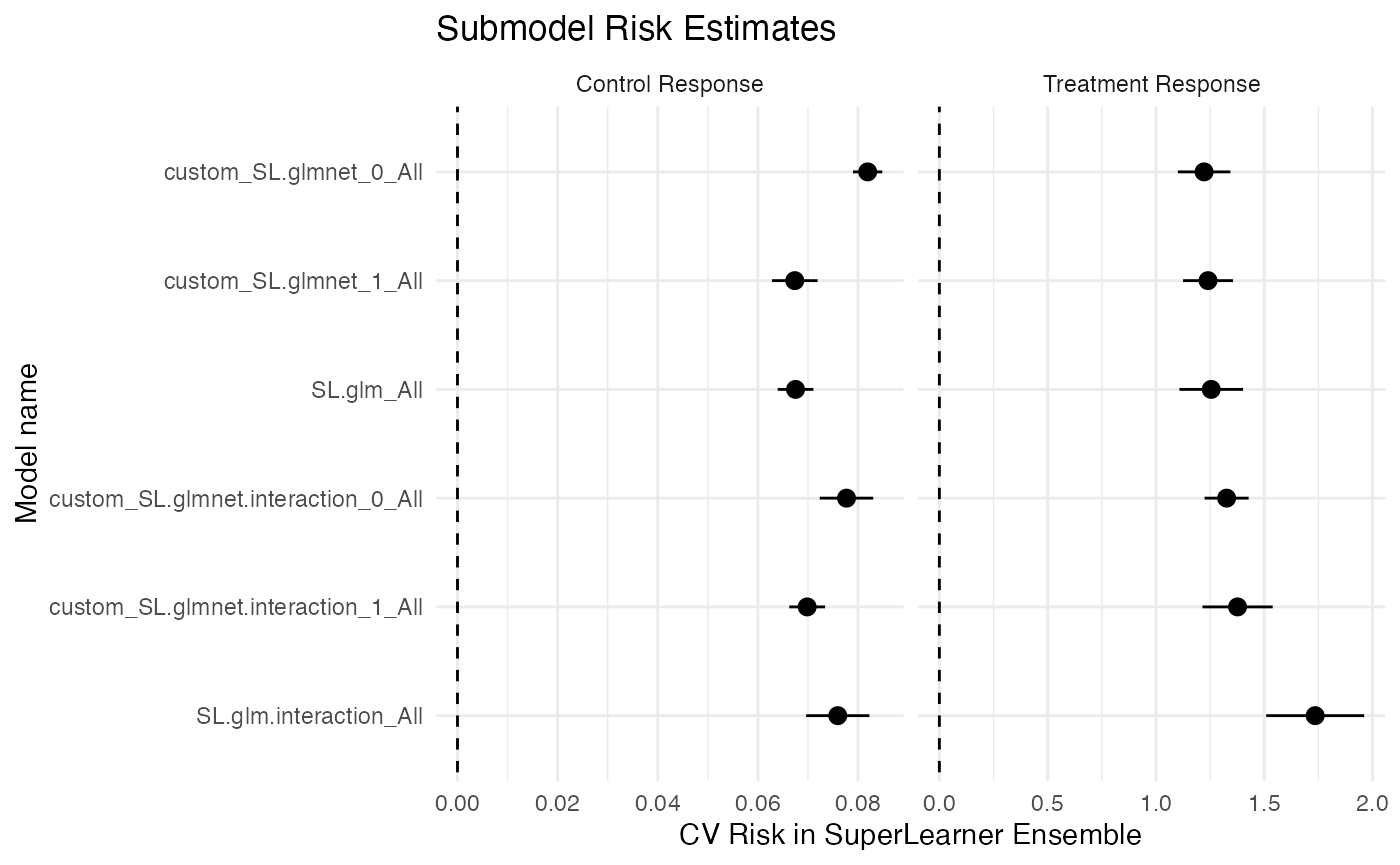
Plot Regression ROC Curves
filter(results, grepl("RROC", estimand)) %>%
  mutate(
    level = factor(level, levels = c("Control Response", "Treatment Response", "Effect Surface"))
  ) %>%
  ggplot() +
  geom_line(
    aes(
      x = value,
      y = estimate
    )
  ) +
  geom_point(
    aes(x = value, y = estimate),
    data = filter(results, grepl("RROC", estimand)) %>% group_by(level) %>% slice_head(n = 1)
  ) +
  expand_limits(y = 0) +
  scale_x_continuous("Over-estimation") +
  scale_y_continuous("Under-estimation") +
  facet_wrap(~level, scales = "free_x") +
  coord_flip() +
  ggtitle("Regression ROC Curves") +
  theme_minimal()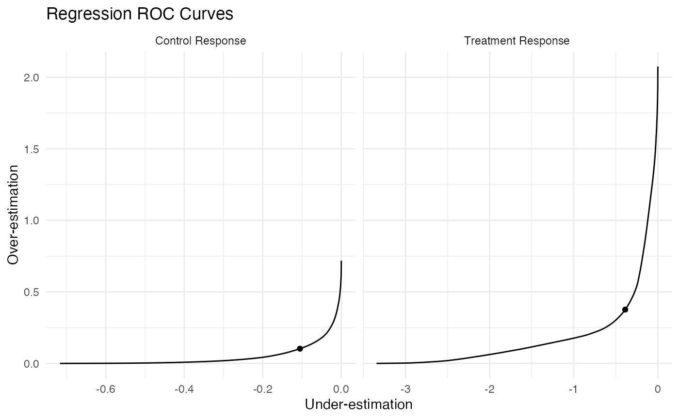
Plot VIMP
ggplot(filter(results, estimand == "VIMP")) +
  geom_abline(intercept = 0, slope = 0, linetype = "dashed") +
  geom_pointrange(
    aes(
      x = term,
      y = estimate,
      ymin = estimate - 1.96 * std_error,
      ymax = estimate + 1.96 * std_error
    )
  ) +
  expand_limits(y = 0) +
  scale_x_discrete("Covariate") +
  scale_y_continuous("Reduction in R² from full model") +
  coord_flip() +
  ggtitle("Covariate Importance") +
  theme_minimal()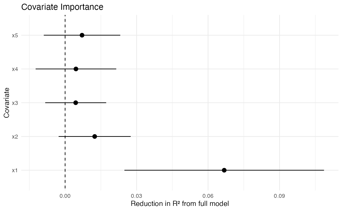
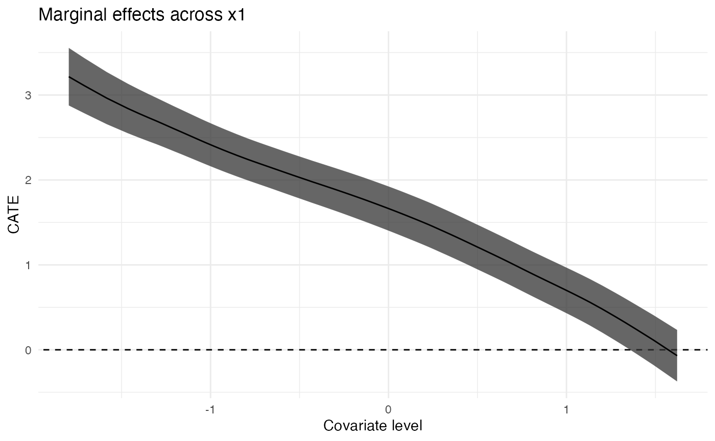
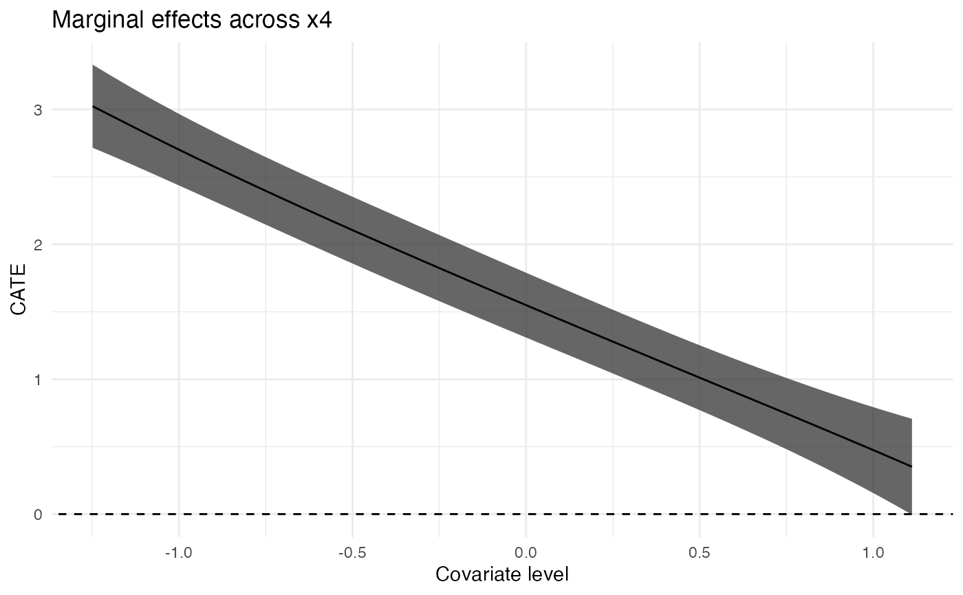
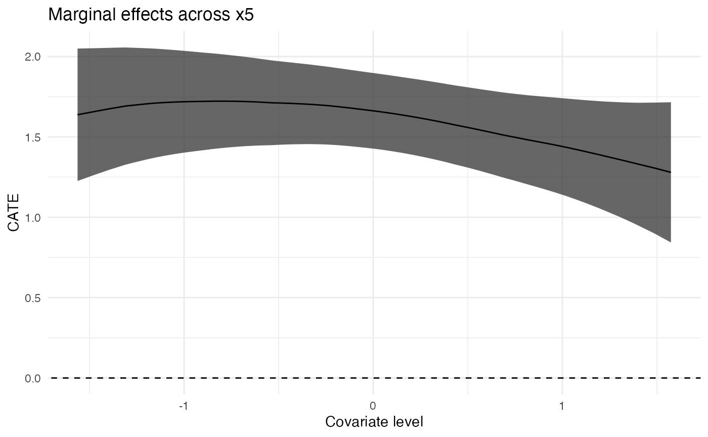
Plot Continuous Covariates’ MCATE
for (cov in c("x1", "x4", "x5")) {
  gp <- ggplot(filter(results, estimand == "MCATE", term == cov)) +
    geom_abline(intercept = 0, slope = 0, linetype = "dashed") +
    geom_ribbon(
      aes(
        x = value,
        ymin = estimate - 1.96 * std_error,
        ymax = estimate + 1.96 * std_error
      ),
      alpha = 0.75
    ) +
    geom_line(
      aes(x = value, y = estimate)
    ) +
    expand_limits(y = 0) +
    scale_x_continuous("Covariate level") +
    scale_y_continuous("CATE") +
    ggtitle(paste("Marginal effects across", cov)) +
    theme_minimal()
  print(gp)
}
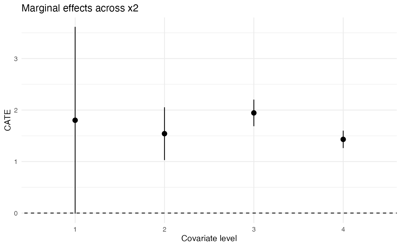
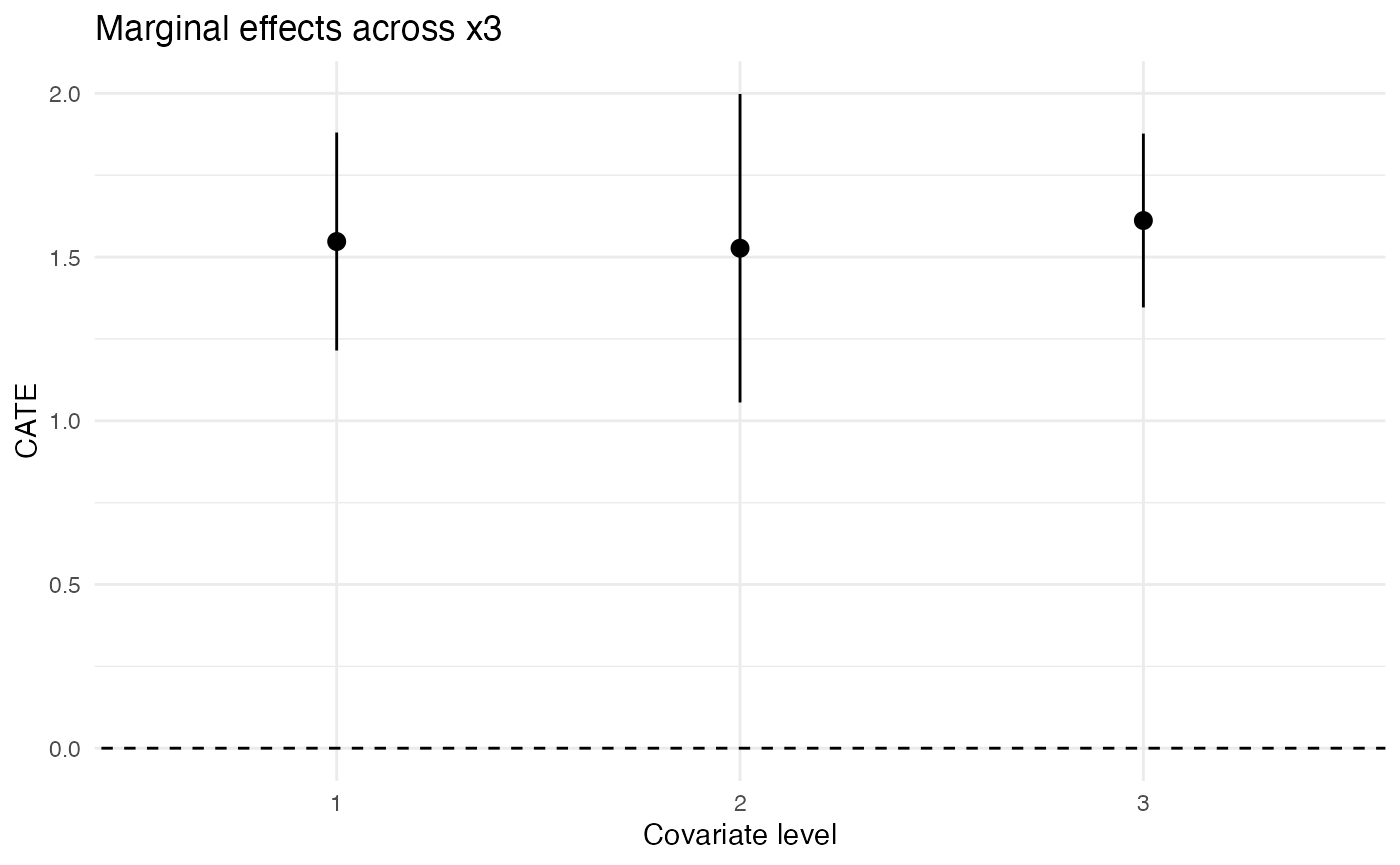
Plot Discrete Covariates’ MCATE
for (cov in c("x2", "x3")) {
  gp <- ggplot(filter(results, estimand == "MCATE", term == cov)) +
    geom_abline(intercept = 0, slope = 0, linetype = "dashed") +
    geom_pointrange(
      aes(
        x = level,
        y = estimate,
        ymin = estimate - 1.96 * std_error,
        ymax = estimate + 1.96 * std_error
      )
    ) +
    expand_limits(y = 0) +
    scale_x_discrete("Covariate level") +
    scale_y_continuous("CATE") +
    ggtitle(paste("Marginal effects across", cov)) +
    theme_minimal()
  print(gp)
}
Session Info
print(sessionInfo())## R version 4.5.1 (2025-06-13)
## Platform: aarch64-apple-darwin20
## Running under: macOS Sequoia 15.6.1
##
## Matrix products: default
## BLAS: /Library/Frameworks/R.framework/Versions/4.5-arm64/Resources/lib/libRblas.0.dylib
## LAPACK: /Library/Frameworks/R.framework/Versions/4.5-arm64/Resources/lib/libRlapack.dylib; LAPACK version 3.12.1
##
## locale:
## [1] en_US.UTF-8/en_US.UTF-8/en_US.UTF-8/C/en_US.UTF-8/en_US.UTF-8
##
## time zone: UTC
## tzcode source: internal
##
## attached base packages:
## [1] stats graphics grDevices utils datasets methods base
##
## other attached packages:
## [1] nnls_1.6 SuperLearner_2.0-29 dplyr_1.1.4
## [4] ggplot2_4.0.0 tidyhte_1.0.4
##
## loaded via a namespace (and not attached):
## [1] vimp_2.3.6 utf8_1.2.6 sass_0.4.10 generics_0.1.4
## [5] quickblock_0.2.2 shape_1.4.6.1 lattice_0.22-7 distances_0.1.12
## [9] hms_1.1.3 digest_0.6.37 magrittr_2.0.4 evaluate_1.0.5
## [13] grid_4.5.1 RColorBrewer_1.1-3 iterators_1.0.14 fastmap_1.2.0
## [17] Matrix_1.7-3 glmnet_4.1-10 foreach_1.5.2 jsonlite_2.0.0
## [21] progress_1.2.3 backports_1.5.0 survival_3.8-3 purrr_1.1.0
## [25] scales_1.4.0 codetools_0.2-20 textshaping_1.0.3 jquerylib_0.1.4
## [29] cli_3.6.5 rlang_1.1.6 crayon_1.5.3 splines_4.5.1
## [33] withr_3.0.2 cachem_1.1.0 yaml_2.3.10 tools_4.5.1
## [37] checkmate_2.3.3 boot_1.3-31 nprobust_0.5.0 vctrs_0.6.5
## [41] R6_2.6.1 lifecycle_1.0.4 fs_1.6.6 htmlwidgets_1.6.4
## [45] MASS_7.3-65 ragg_1.5.0 pkgconfig_2.0.3 desc_1.4.3
## [49] pkgdown_2.1.3 pillar_1.11.1 bslib_0.9.0 gtable_0.3.6
## [53] glue_1.8.0 data.table_1.17.8 Rcpp_1.1.0 systemfonts_1.3.1
## [57] xfun_0.53 tibble_3.3.0 tidyselect_1.2.1 knitr_1.50
## [61] farver_2.1.2 htmltools_0.5.8.1 labeling_0.4.3 rmarkdown_2.30
## [65] gam_1.22-6 compiler_4.5.1 quadprog_1.5-8 prettyunits_1.2.0
## [69] S7_0.2.0